Generative Psychometrics: Measurement Theory for Self-Reflective Constructs

Abstract

The Generative Measurement Model (GMM) is a psychometric framework in which the measurand is a probability distribution over self-model parameters rather than a latent point. Drawing on the predictive-processing account of identity (Morrison, 2026b), where items function as structured prediction-error generators that simultaneously measure and modify the self-model, three contributions follow. First, a likelihood in which responses marginalise over a person-specific identity distribution $\mathit{\pi}_{\mathit{i}}$(θ) with distributional parameters (location $\mathit{\mu}_{\mathit{i}}$, width ${\mathit{\sigma}_{\mathit{i}}}^{2}$) as primary estimands, and a state-transition equation coupling measurement to self-model revision through metacognitive precision $\mathit{\kappa}_{\mathit{i}}$ and item identity-relevance weights $\mathit{w}_{\mathit{j}}$; Model A (static) is estimable via data-augmentation MCMC, Model B (sequential) requires particle MCMC and remains theoretical. Second, a proof that classical 2PL IRT is a degenerate special case when posterior width and item weights both approach zero; relaxing either yields testable departures. Third, a distributional reliability framework partitioning variability into between-person location, within-person breadth (ontological), and residual error, resolving the paradox that low-reliability instruments may capture real distributional signal. The framework predicts within-occasion consistency exceeds between-occasion consistency under the single-draw-per-occasion assumption, confirmed at 2.34:1 (95% CI [2.10, 2.75]; Morrison, 2026g) and holding in all seven countries with computable retest data. Empirical testing motivates revising κ from scalar update-rate to precision-as-investment with a matrix extension. The κ-alpha discriminator (within-factor-variance consistency) distinguishes simulated GMM from simulated IRT responding (GMM α = .664, IRT α = −.014; 100% power at N = 100), whereas within-factor Cronbach’s alpha over repeat sessions of sixteen language models, negative in 50 of 80 model–factor combinations, has no between-person variance in its input and does not separate the GMM from IRT, so that test needs a design across instances. The framework is domain-restricted to self-reflective constructs; for ability constructs, IRT remains more parsimonious.

Keywords: generative measurement model, distributional measurement, item response theory, metacognitive precision, measurement reactivity, self-reflective constructs, Bayesian psychometrics, distributional reliability, adaptive testing, identity distribution

1. Introduction: The Passivity Assumption in Psychometrics

The entire edifice of modern psychometric theory rests upon an assumption so fundamental that it is rarely stated, let alone interrogated. This assumption, which the present paper terms the ‘passivity assumption,’ holds that measurement is a form of passive observation, so that the act of administering a test leaves the attribute under measurement undisturbed. The assumption pervades classical test theory, item response theory, and the structural equation modelling tradition alike. It is encoded in the very notation of the discipline, where θ denotes a fixed person parameter and X denotes a random variable whose distribution is conditionally determined by θ. The directionality is strictly one-way, from latent attribute to observed response, and the possibility that observed responses might feed back into the latent attribute is excluded by construction. For a substantial class of psychological constructs, the passivity assumption is approximately correct, and its adoption is scientifically productive. For another class, it is not merely incorrect but actively misleading, generating a systematic pattern of anomalies that the discipline has struggled to resolve within its existing theoretical apparatus.

The distinction corresponds to a difference in the relationship between the measured construct and the person’s self-model. Ability constructs, such as fluid intelligence, working memory capacity, and perceptual speed, exist largely independent of the person’s beliefs about them. A person who scores 115 on a matrix reasoning test does not thereby change their matrix reasoning capacity. The measurement is, to a close approximation, non-reactive in the sense articulated by Webb, Campbell, Schwartz & Sechrest (1966), who first systematised the conditions under which observation alters the phenomenon observed. Their taxonomy of reactive measurement effects, developed primarily for behavioural observation in social settings, has received surprisingly little attention within psychometric theory proper, despite its direct relevance to the formal properties of psychological measurement. The passivity assumption amounts to the claim that psychometric measurement is non-reactive, and for ability constructs this claim is defensible. One’s capacity for spatial rotation is not altered by being asked to rotate objects mentally, at least not within the timescale of a single testing occasion, although practice effects across occasions constitute an important qualification addressed below.

Self-reflective constructs present an entirely different situation. When a person responds to the item ‘I see myself as someone who is organised and likes to keep things tidy,’ the response is not a passive readout of a fixed organisational tendency. It is the product of an inferential process in which the person consults their self-model, generates a prediction about their own behaviour, compares that prediction against available autobiographical evidence, and produces a response that reflects the outcome of this comparison. The critical observation, developed at length in Morrison (2026b), is that this inferential process can itself update the self-model. If the comparison reveals a discrepancy between the self-model’s prediction and the retrieved evidence, the resulting prediction error constitutes information that the self-model may assimilate. The act of responding to the item has generated a perturbation in the very attribute the item was designed to measure. Consequently, the measurement of a self-reflective construct amounts to an intervention upon it.

This claim is philosophical, and it is also empirical, as it generates a distinctive pattern of predictions that correspond to well-documented anomalies in the personality measurement literature. Firstly, the replication crisis in personality psychology is predicted if measurement occasions alter the distributions from which responses are drawn, shifting participants’ distributions before they encounter any experimental manipulation. Secondly, practice effects in personality assessment are predicted if repeated measurement generates cumulative self-model updates. Thirdly, item order effects (different item sequences producing different parameter estimates) are predicted if earlier items generate prediction errors that update the self-model before later items are encountered. Standard IRT predicts no order effects whatsoever. Lastly, the characteristically lower test-retest reliability of identity-relevant measures is predicted if the first testing occasion generates self-model updates whose magnitude varies across individuals.

The present paper develops a formal measurement theory for the case where the passivity assumption fails. This theory, termed the GMM, treats the person parameter not as a fixed point but as a distribution, $\mathit{\pi}_{\mathit{i}}$(θ), parameterised by distributional parameters $\mathit{\varphi}_{\mathit{i}}$, and introduces a state transition mechanism through which measurement occasions can update this distribution. The framework makes three novel contributions. The first is a formal state transition equation that couples measurement and state change within a single model. In existing dynamic measurement models such as van Rijn, Dolan & Molenaar (2010) and LaMar (2018), measurement and transition equations are formally independent, meaning measurement itself cannot cause state change. The GMM’s transition equation makes measurement an explicit cause of state change, with the magnitude governed by item and person parameters.

The second contribution is the treatment of asymptotic posterior width, ${\mathit{\sigma}_{\mathit{i}}}^{2}$, as a substantive person parameter rather than as estimation error to be minimised. In standard IRT, the posterior variance of $\mathit{\theta}_{\mathit{i}}$ reflects uncertainty in the estimate of a fixed quantity. As the number of items increases, this variance shrinks toward zero, and its rate of shrinkage is the primary concern of measurement precision. In the GMM, ${\mathit{\sigma}_{\mathit{i}}}^{2}$ reflects the genuine width of the person’s identity distribution – a psychologically meaningful individual difference. A person with large ${\mathit{\sigma}_{\mathit{i}}}^{2}$ is not poorly measured. They have a wide distribution over the construct in question, reflecting either identity exploration, contextual variability, or both. This parameter does not vanish with additional items. It stabilises at a non-zero asymptote that characterises the person. Ferrando (2016) develops the most direct antecedent to this claim within the IRT tradition, introducing person discriminal dispersion (PDD) as an individual-difference parameter capturing response variability; Section 2.6 engages substantively with the relationship between PDD and ${\mathit{\sigma}_{\mathit{i}}}^{2}$. Embretson (1991) anticipated further aspects of the distributional claim in demonstrating that learning during testing produces systematic changes in ability parameters, although she did not develop a distributional measurement framework for the person parameters themselves.

The third contribution is $\mathit{\kappa}_{\mathit{i}}$, a continuous person parameter representing the metacognitive channel through which measurement-induced prediction errors are assimilated into the self-model. A person with $\mathit{\kappa}_{\mathit{i}}$ near zero is metacognitively opaque to the measurement process, so that item responses generate prediction errors that are not integrated into the self-model. A person with $\mathit{\kappa}_{\mathit{i}}$ near one is maximally transparent, assimilating prediction errors fully. This parameter provides a formal account of individual differences in reactivity to measurement, a phenomenon well-documented empirically but lacking a measurement-theoretic formalisation. Dayan (2023) develops an information-theoretic account of metacognitive precision that provides independent theoretical grounding for $\mathit{\kappa}_{\mathit{i}}$, although Dayan’s framework addresses perceptual metacognition rather than the self-reflective metacognition at issue here.

Three qualifications bound the scope of this contribution. Firstly, the GMM is designed for self-reflective constructs and does not compete with IRT for ability measurement. The domain boundary is continuous, operationalised by the average $\mathit{w}_{\mathit{j}}$ across items. When average $\mathit{w}_{\mathit{j}}$ approaches zero, the GMM reduces to standard IRT. Secondly, Model A (static, within-occasion) is fully estimable and constitutes the paper’s primary empirical contribution. Model B (sequential, incorporating the state transition equation) requires particle MCMC and is deferred. Lastly, the GMM recovers standard 2PL IRT as a degenerate special case when ${\mathit{\sigma}_{\mathit{i}}}^{2}$ approaches zero and $\mathit{w}_{\mathit{j}}$ equals zero for all items, in which case $\mathit{\kappa}_{\mathit{i}}$ becomes irrelevant since $\mathit{\kappa}_{\mathit{i}}$ · $\mathit{w}_{\mathit{j}}$ vanishes regardless of $\mathit{\kappa}_{\mathit{i}}$’s value. This subsumption result (Section 2.5) establishes the GMM as a strict generalisation of the 2PL.

The paper proceeds as follows. Section 2 develops the formal GMM, presenting the likelihood function, state transition equation, estimation procedure, identifiability analysis, the IRT subsumption theorem, and engagement with existing measurement frameworks. Section 3 develops the distributional reliability framework. Section 4 develops the item taxonomy and adaptive testing under GMM. Section 5 derives the replication crisis predictions and reconciles the framework with Big Five stability. Section 6 presents the empirical programme, including a parameter recovery simulation, a planned re-analysis of existing test-retest data, and three proposed experimental studies. Section 7 develops trajectory validity as the appropriate validity concept for reactive measurement. Section 8 engages objections. Section 9 concludes.

2. The GMM

The GMM is built upon a single foundational departure from standard IRT. Where IRT treats person i’s latent trait value as a fixed point $\mathit{\theta}_{\mathit{i}}$, the GMM treats it as a random variable drawn from a person-specific identity distribution $\mathit{\pi}_{\mathit{i}}$(θ), parameterised by distributional parameters $\mathit{\varphi}_{\mathit{i}}$ (Figure 1). For a Beta-distributed construct scaled to [0, 1], $\mathit{\varphi}_{\mathit{i}}$ = ($\mathit{\alpha}_{\mathit{i}}$, $\mathit{\beta}_{\mathit{i}}$), from which one can derive the distributional mean $\mathit{\mu}_{\mathit{i}}$ = $\mathit{\alpha}_{\mathit{i}}$/($\mathit{\alpha}_{\mathit{i}}$ + $\mathit{\beta}_{\mathit{i}}$) and variance ${\mathit{\sigma}_{\mathit{i}}}^{2}$ = $\mathit{\alpha}_{\mathit{i}}$·$\mathit{\beta}_{\mathit{i}}$/(($\mathit{\alpha}_{\mathit{i}}$ + $\mathit{\beta}_{\mathit{i}}$)²($\mathit{\alpha}_{\mathit{i}}$ + $\mathit{\beta}_{\mathit{i}}$ + 1)). The key substantive claim is that ${\mathit{\sigma}_{\mathit{i}}}^{2}$ is not estimation uncertainty but a genuine person parameter reflecting the width of the individual’s identity distribution on the construct in question. This section develops the formal apparatus.

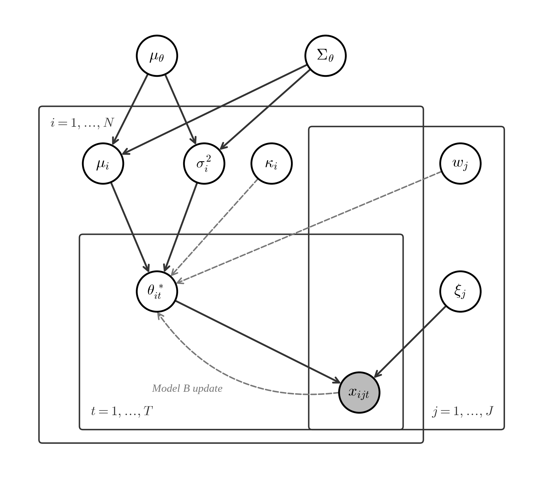
Figure 1. Plate diagram for the GMM. Shaded node indicates observed variable, the response $\mathit{x}_{\mathit{i}\ \mathit{j}\ \mathit{t}}$ of person i to item j on occasion t. Population parameters (mean $\mathit{\mu}_{\mathit{\theta}}$ and covariance $\mathit{\Sigma}_{\mathit{\theta}}$) generate person-specific identity distributions, from which occasion-specific draws produce item responses. Dashed arrows indicate the Model B state transition (measurement-as-intervention), in which each response updates the identity distribution behind later draws with weight $\mathit{\kappa}_{\mathit{i}}$ · $\mathit{w}_{\mathit{j}}$.

2.1 The Likelihood Function

Consider person i responding to items j = 1, …, J on a single measurement occasion. Each item is characterised by item parameters $\mathit{\xi}_{\mathit{j}}$, which under the 2PL parameterisation consist of discrimination $\mathit{a}_{\mathit{j}}$ and difficulty $\mathit{b}_{\mathit{j}}$. The standard 2PL item response function gives the probability of a correct or endorsed response conditional on the latent trait value.

The GMM’s Model A likelihood rests on what the paper terms the ‘single-draw-per-occasion’ assumption. On any given measurement occasion, person i draws a single value $\mathit{\theta}^{\mathit{\ast}}$ from their identity distribution $\mathit{\pi}_{\mathit{i}}$(θ | $\mathit{\varphi}_{\mathit{i}}$), and all J item responses on that occasion are conditionally independent given this single draw. The marginal likelihood, obtained by integrating over the unobserved draw, takes the form

$$\mathit{L}_{\mathit{A}}\left( \mathit{\varphi}_{\mathit{i}},\ \mathit{\xi}\ |\ \mathit{x}_{\mathit{i}} \right)\ = \ \int_{}^{}{\ \prod_{\mathit{j} = 1}^{\mathit{J}}{\ \mathit{P}\left( \mathit{X}_{\mathit{ij}}\ = \ \mathit{x}_{\mathit{ij}}\ |\ \mathit{\theta},\ \mathit{\xi}_{\mathit{j}} \right)\ \cdot \ \mathit{\pi}\left( \mathit{\theta}\ |\ \mathit{\varphi}_{\mathit{i}} \right)\ \mathit{d\theta}.}}$$

The integral falls outside the product, which is the defining structural feature of Model A and the source of its distinctive predictions. This placement has a precise substantive interpretation. On a given occasion, the person occupies a single location on the construct, drawn from their identity distribution, and all responses on that occasion reflect this single location. The within-occasion responses are therefore correlated beyond what is predicted by the marginal response probabilities, because they share a common latent draw. Between occasions, however, fresh draws from $\mathit{\pi}_{\mathit{i}}$(θ) are independent (conditional on $\mathit{\varphi}_{\mathit{i}}$), and so between-occasion responses exhibit lower correlation.

This likelihood structure produces a testable prediction that standard IRT cannot generate. Under standard IRT with fixed $\mathit{\theta}_{\mathit{i}}$, the correlation structure of responses is fully determined by the item parameters and the single fixed trait value. There is no mechanism by which within-occasion consistency could systematically exceed between-occasion consistency once item parameters are controlled. Under Model A, this dominance is a structural consequence of the single-draw assumption (Figure 2). Within an occasion, responses share a common $\mathit{\theta}^{\mathit{\ast}}$, and their residual correlations (after conditioning on $\mathit{\varphi}_{\mathit{i}}$ but not on $\mathit{\theta}^{\mathit{\ast}}$) are positive. Between occasions, responses are drawn from independent realisations of $\mathit{\theta}^{\mathit{\ast}}$, and their residual correlations (after conditioning on $\mathit{\varphi}_{\mathit{i}}$) reflect only the shared distributional parameters. The magnitude of the within-versus-between consistency gap is a monotonically increasing function of ${\mathit{\sigma}_{\mathit{i}}}^{2}$, which provides a direct empirical indicator of the identity distribution width.

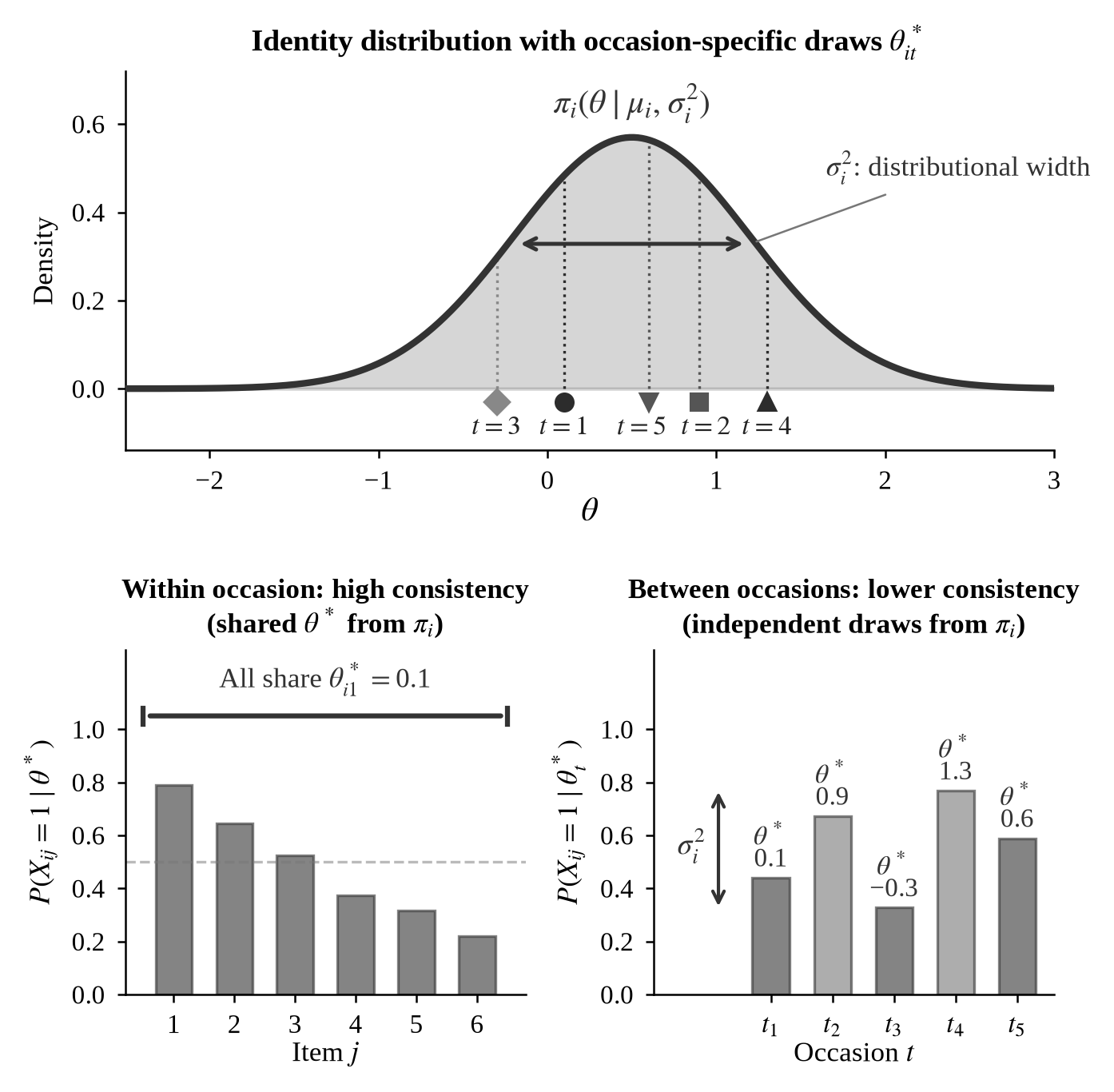
Figure 2. The single-draw-per-occasion assumption generates the within > between prediction. Upper panel shows the identity distribution with occasion-specific draws. Lower-left panel shows that within an occasion, all items share a common draw, producing high consistency. Lower-right panel shows that between occasions, independent draws from the identity distribution introduce variation governed by distributional width.

The prediction that within-occasion consistency exceeds between-occasion consistency has been confirmed with a ratio of approximately 2.34:1 across all five Big Five factors in the IPIP‑FFM dataset (N ≈ 100,000; Morrison, 2026g), with 95% bootstrap confidence interval [2.10, 2.75] from 10,000 resamples firmly excluding unity. The result is reproducible only when $\mathit{\sigma}_{\mathit{\kappa}}$ (the between-person spread of distributional breadth in the simulation calibration) exceeds zero. Under that condition, the distributional framework is empirically necessary, as standard IRT with fixed trait values cannot generate the effect. Seven adversarial controls (same-person validation, copy-paste detection, temporal decay, screen relaxation, random pairing, simulation calibration, and response time consistency) confirm the robustness of the finding, with the minimum factor-level ratio at 1.51 (Openness) and significant heterogeneity across subgroups ($\mathit{I²}$ = 77–99%) that nonetheless preserves the ratio above unity in every cell.

The single-draw-per-occasion assumption is strong, and one might argue that a person’s effective trait level fluctuates within an occasion. The assumption is best understood as an idealisation that becomes more accurate as occasion duration decreases, and the model’s fit to data provides an empirical test of its adequacy. The present paper retains it for parsimony and because the resulting model is already sufficient to generate novel predictions.

The relationship between Model A and Fox’s (2010) random-effects IRT framework warrants careful articulation, since the two share formal similarities that might obscure their substantive differences. Fox develops an hierarchical Bayesian IRT model in which person parameters $\mathit{\theta}_{\mathit{i}}$ are drawn from a population distribution, typically normal, with hyperparameters governing the population mean and variance. The person-specific prior in Fox’s framework represents population-level variability, in that different people occupy different locations on the construct, and the prior’s variance reflects between-person heterogeneity. In the GMM, the person-specific distribution $\mathit{\pi}_{\mathit{i}}$(θ | $\mathit{\varphi}_{\mathit{i}}$) represents within-person variability, in that the same person occupies different locations across occasions. The formal likelihood has the same structure (the conditional likelihood is integrated against a prior), but the referent of the integration variable is fundamentally different. In Fox’s model, integrating over θ marginalises out uncertainty about a fixed person parameter. In Model A, integrating over θ marginalises out the within-person variation constituting the phenomenon of interest.

This distinction has consequences for estimation. In Fox’s framework, as the number of items increases, the posterior for $\mathit{\theta}_{\mathit{i}}$ concentrates around the true fixed value, and the prior’s contribution diminishes. In Model A, increasing the number of items within an occasion concentrates the posterior for the occasion-specific draw $\mathit{\theta}^{\mathit{\ast}}$, but the distributional parameters $\mathit{\varphi}_{\mathit{i}}$ are estimated from the pattern of variation across occasions. The data structure required for Model A estimation is therefore multi-occasion data in which the same person responds to the same (or linked) items on multiple occasions, a design common in longitudinal personality research but rarely analysed with the distributional focus the GMM motivates.

2.2 The State Transition Equation

Model A captures the consequences of distributional person parameters for measurement but does not formally represent the mechanism by which measurement changes the distribution. Model B introduces a state transition equation that makes measurement-as-intervention explicit.

Under Model B, the identity distribution updates sequentially within an occasion as each item is encountered. After person i responds to item j with observed response $\mathit{x}_{\mathit{ij}}$, the identity distribution updates according to

$$\mathit{\pi}_{\mathit{i}}^{\left( \mathit{j} + 1 \right)}\left( \mathit{\theta} \right)\ \propto \ \mathit{\pi}_{\mathit{i}}^{\left( \mathit{j} \right)}\left( \mathit{\theta} \right)\ \cdot \ \mathit{P}\left( \mathit{x}_{\mathit{ij}}\ |\ \mathit{\theta} \right)^{\mathit{\kappa}_{\mathit{i}}\ \cdot \ \mathit{w}_{\mathit{j}}}$$

where $\mathit{\pi}_{\mathit{i}}^{(1)}$(θ) = π(θ | $\mathit{\varphi}_{\mathit{i}}$) is the initial distribution, $\mathit{\kappa}_{\mathit{i}}$ ∈ [0, 1] is the person-specific metacognitive channel parameter, and $\mathit{w}_{\mathit{j}}$ ∈ [0, 1] is the item identity-relevance weight. The update is formally a tempered Bayesian update, in which the likelihood contribution of item j is raised to the power $\mathit{\kappa}_{\mathit{i}}$ · $\mathit{w}_{\mathit{j}}$ before being absorbed into the prior for item j + 1.

This equation is formally distinct from all existing dynamic measurement models in one specific respect. In state-space models of the kind developed by van Rijn, Dolan & Molenaar (2010) and others, the measurement equation $\mathit{P}\left( \mathit{X}_{\mathit{t}}\ |\ \mathit{\theta}_{\mathit{t}} \right)$ and the transition equation $\mathit{P}\left( \mathit{\theta}_{\mathit{t} + 1}\ |\ \mathit{\theta}_{\mathit{t}} \right)$ are separate, with the transition equation governing how the latent state evolves due to processes other than measurement, such as development, learning, or environmental change. The measurement equation maps the current state to observed responses, but measurement itself does not appear as a term in the transition equation. In Model B, the transition equation is the measurement equation, tempered by $\mathit{\kappa}_{\mathit{i}}$ and $\mathit{w}_{\mathit{j}}$. The act of producing a response to item j is what drives the state change. This coupling formalises the claim that measurement is intervention for self-reflective constructs.

The parameters $\mathit{\kappa}_{\mathit{i}}$ and $\mathit{w}_{\mathit{j}}$ govern the magnitude of the coupling. When $\mathit{\kappa}_{\mathit{i}}$ = 0, the person is metacognitively opaque and no measurement-induced updating occurs, regardless of item content. When $\mathit{w}_{\mathit{j}}$ = 0, the item has no identity relevance and produces no updating regardless of the person’s metacognitive transparency. The product $\mathit{\kappa}_{\mathit{i}}$ · $\mathit{w}_{\mathit{j}}$ determines the effective strength of the measurement-as-intervention effect for person i on item j. Note that when both $\mathit{\kappa}_{\mathit{i}}$ = 0 and $\mathit{w}_{\mathit{j}}$ = 0 hold globally, the state transition equation reduces to $\mathit{\pi}_{\mathit{i}}^{\left( \mathit{j} + 1 \right)}$(θ) ∝ $\mathit{\pi}_{\mathit{i}}^{\left( \mathit{j} \right)}$(θ) · $\mathit{P}\left( \mathit{x}_{\mathit{ij}}\ |\ \mathit{\theta} \right)^{0}$ = $\mathit{\pi}_{\mathit{i}}^{\left( \mathit{j} \right)}$(θ), and no updating occurs. This is one of the conditions under which the GMM reduces to standard IRT.

Model B’s sequential updating introduces a likelihood inconsistency relative to Model A, because Model A treats all J responses as conditionally independent given a single draw while Model B implies the distribution changes after each item. The two likelihoods are formally incompatible. Model A is presented as the estimable primary model; Model B is the theoretical extension with estimation via particle MCMC deferred to future work. Even within Model A, however, measurement-as-intervention is captured at the between-occasion level, as distributional parameters $\mathit{\varphi}_{\mathit{i}}^{\left( \mathit{t} \right)}$ may change across occasions as a function of the measurement occasions themselves.

Empirical testing of the state transition equation’s predictions has motivated a substantive revision of the interpretation of $\mathit{\kappa}_{\mathit{i}}$. The original formulation treats $\mathit{\kappa}_{\mathit{i}}$ as a scalar update-rate parameter, such that high-$\mathit{\kappa}_{\mathit{i}}$ individuals assimilate measurement-generated prediction errors more fully and therefore revise their self-models more extensively in response to identity-relevant items. Under this interpretation, high $\mathit{\kappa}_{\mathit{i}}$ combined with high $\mathit{w}_{\mathit{j}}$ should produce maximal retest instability on identity-relevant items. Item-level analysis of retest data (N = 1,030 retest pairs, 50 items; Morrison, 2026g) disconfirms this prediction in a specific and informative manner. The $\mathit{\kappa}_{\mathit{i}}$ × $\mathit{w}_{\mathit{j}}$ interaction is statistically significant (β = −0.031, p = .013 in multilevel modelling) but operates in the opposite direction from the update-rate interpretation, as high-$\mathit{\kappa}_{\mathit{i}}$ individuals show less retest instability on high-$\mathit{w}_{\mathit{j}}$ items, not more. The main effect of cross-factor response variance (the $\mathit{\kappa}_{\mathit{i}}$ proxy, which Section 2.4 reports as capturing distributional width) on overall retest variability remains robust (β = 0.186, p < 10⁻¹⁰, positive for all 50 items), confirming that persons high on the proxy are more variable in their responses overall. The conjunction of these two findings (greater overall variability but selective stability on identity-relevant items) is inconsistent with precision-as-update-rate but consistent with precision-as-investment, whereby $\mathit{\kappa}_{\mathit{i}}$ indexes the selective allocation of precision resources to identity-relevant dimensions rather than a uniform update rate applied indiscriminately across all dimensions.

The precision-as-investment interpretation reconceives $\mathit{\kappa}_{\mathit{i}}$ as governing which dimensions receive preferential precision allocation rather than the rate at which all dimensions are updated. This reinterpretation was generated post hoc in response to the wrong-direction $\mathit{\kappa}_{\mathit{i}}$ × $\mathit{w}_{\mathit{j}}$ interaction of Prediction 5 (Section 9.3) and accordingly requires prospective confirmation from the P‑KAI predictions developed below before it can be treated as established rather than provisional. Under this account, a person with high $\mathit{\kappa}_{\mathit{i}}$ invests precision resources disproportionately in dimensions central to their functional self-model, thereby protecting those dimensions from perturbation while remaining more variable on peripheral dimensions. Three converging lines of evidence support this reinterpretation. Firstly, the wrong-direction interaction at item level (β = −0.031, p = .013) directly disconfirms uniform update-rate and supports selective protection. Secondly, perturbation dose-response in synthetic systems is linear rather than sigmoidal (linear AIC preferred in all six model-dimension combinations; Morrison, 2026g), consistent with proportional resource allocation rather than threshold-based prior resistance. Thirdly, the collapse of the variance-shift correlation from r = 0.548 at ten dimensions to r = 0.127 at twenty dimensions (Morrison, 2026g) demonstrates that perturbation susceptibility corresponds to training prior strength rather than output variance, further supporting the interpretation that precision is invested selectively rather than distributed uniformly. Of these three converging lines, only the first derives from human psychometric data, while the second and third are from synthetic systems whose relationship to human self-model dynamics remains an open empirical question. The human evidence alone (the item-level interaction) is suggestive but not independently decisive, and the P‑KAI predictions below must be borne out before the precision-as-investment interpretation can be regarded as established.

The precision-as-investment interpretation has formal consequences for the state transition equation. Where the original formulation specifies a scalar $\mathit{\kappa}_{\mathit{i}}$ applied uniformly across all items, the revised formulation motivates a matrix extension $\mathit{K}_{\mathit{i}}$ = [$\mathit{K}_{\mathit{i},\mathit{jk}}$] giving dimension-specific and item-specific precision allocation, such that the effective update for person i on item j is governed by $\mathit{K}_{\mathit{i},\mathit{jj}}$ · $\mathit{w}_{\mathit{j}}$ rather than $\mathit{\kappa}_{\mathit{i}}$ · $\mathit{w}_{\mathit{j}}$. The total precision budget, Trace($\mathit{K}_{\mathit{i}}$), is constrained by a finite metacognitive resource, and the distribution of precision across dimensions (the shape of the allocation profile) becomes a second-order person parameter characterising how, rather than how much, an individual invests in self-model maintenance. This extension preserves the IRT subsumption result, as $\mathit{K}_{\mathit{i},\mathit{jj}}$ = 0 for all i, j yields the same degenerate case as $\mathit{\kappa}_{\mathit{i}}$ = 0, but generates richer predictions about the relationship between identity structure and measurement dynamics. The matrix extension is presented here as a theoretical refinement motivated by empirical findings; its estimation requires substantially richer data than the scalar formulation and is deferred to future work.

The matrix extension generates three novel predictions (designated P‑KAI1 through P‑KAI3) that are jointly specific to the precision-as-investment interpretation and cannot be derived from the scalar formulation or from standard IRT.

P‑KAI1 concerns the selectivity of retest stability under high precision investment. If $\mathit{K}_{\mathit{i},\mathit{jj}}$ is proportional to the factor loading $\mathit{\lambda}_{\mathit{j}}$ for dimension j, then individuals with high Trace(K) (high total precision investment) should concentrate their precision resources on dimensions where the factor structure is strongest. The empirical consequence is that high-Trace(K) individuals should exhibit lower retest change specifically on items with high factor loadings, while showing equal or higher retest change on items with low factor loadings. Under the scalar formulation, high $\mathit{\kappa}_{\mathit{i}}$ predicts either uniform stability (if κ indexes resistance) or uniform instability (if κ indexes update rate) across all items regardless of their loading magnitude. The matrix formulation predicts a crossover interaction whereby precision investment is selective rather than uniform, concentrated where the identity distribution’s factor structure provides the strongest signal. This prediction is testable with existing IPIP‑FFM retest data by computing item-level factor loadings, splitting items by loading magnitude, and comparing retest change across high versus low Trace(K) terciles estimated from cross-factor variance.

P‑KAI2 concerns the population-level correspondence between precision allocation and factor structure. If K is shaped by accumulated experience with factor-coherent item sets, with individuals learning to invest precision where the empirical covariance structure rewards such investment, then the diagonal of K should correlate with the empirical factor loading pattern at the population level. Individuals should, on average, invest more precision in dimensions with higher factor loadings, producing a positive rank-order correlation between $\mathit{K}_{\mathit{jj}}$ and $\mathit{\lambda}_{\mathit{j}}$ across dimensions. This prediction is testable using response time dynamics as a proxy for the diagonal of K. Within-factor RT acceleration slope (the rate at which response times decrease across successive items tapping the same factor) serves as a behavioural index of precision accumulation on that dimension. P‑KAI2 predicts a positive correlation between this slope and the corresponding factor loading, such that dimensions with stronger factor structure elicit steeper RT acceleration as the system invests precision more efficiently where the signal is clearest. The scalar formulation, which treats $\mathit{\kappa}_{\mathit{i}}$ as uniform across dimensions, cannot generate this dimension-specific prediction.

P‑KAI3 concerns the interaction of precision investment with dimension familiarity. Under the matrix extension, $\mathit{K}_{\mathit{i},\mathit{jj}}$ ≈ 0 for novel or unfamiliar dimensions on which the individual has had no opportunity to accumulate precision investment. Perturbation resistance on such dimensions should therefore reduce to a baseline level regardless of the individual’s overall precision budget Trace(K). The prediction is that κ should predict perturbation resistance on familiar dimensions but not on novel dimensions, producing a significant κ × familiarity interaction on perturbation resistance. This prediction is directly testable by crossing the novel-dimensions protocol (Morrison, 2026g), which assesses synthetic system responses on both familiar Big Five dimensions and fabricated novel dimensions, with a κ proxy derived from familiar-dimension variance. On familiar dimensions, high-κ systems should resist perturbation more effectively; on novel dimensions, where no prior precision investment exists, κ should be non-predictive. The scalar formulation predicts that κ should predict resistance uniformly across all dimensions regardless of familiarity, a prediction that the collapse of the posterior-inertia signature (S1) at twenty dimensions (Morrison, 2026g) has already rendered implausible.

These three predictions are jointly specific to the matrix extension of the precision-as-investment interpretation. Their confirmation would establish that κ operates as a structured allocation profile rather than a scalar parameter, with implications for both psychometric assessment design and the operational measurement of self-model maintenance in artificial systems. Their disconfirmation, particularly if high-Trace(K) individuals show uniform rather than selective stability across loading magnitudes (contra P‑KAI1), would indicate that precision investment, although directionally correct as an interpretation of the P5 finding, does not require the full matrix apparatus.

P‑KAI1 has been tested directly against the IPIP‑FFM retest data (N = 1,030 pairs, 50 items; Morrison, 2026g). The result is not supported. The person-level interaction between total precision investment (estimated via cross-factor variance) and loading magnitude yields a null coefficient (β = +0.003, p = .877), and the item-level operationalisation yields a significant but oppositely signed coefficient (β = +0.013, p = .008) relative to the P5 finding (β = −0.031, p = .013) on which the precision-as-investment interpretation was originally grounded. The discrepancy between the two item-level operationalisations (loading-based versus item-weight-based selectivity) suggests that the selectivity pattern is sensitive to how item importance is operationalised, a finding that does not falsify the matrix extension but constrains the conditions under which selective protection manifests. The 95% bootstrap confidence interval for the person-level interaction spans zero (−0.014 to +0.020), and three of five factors show negative coefficients without individual significance. P‑KAI2 and P‑KAI3 have not yet been tested. On present evidence, the precision-as-investment interpretation generates productive theoretical consequences but does not yet have robust prospective confirmation from its own novel predictions.

2.3 Estimation

Model A can be estimated using data augmentation Markov chain Monte Carlo, a well-established strategy in Bayesian IRT (Albert, 1992; Fox, 2010). The estimation proceeds in alternating steps.

In Step 1, for each person i and occasion t, the occasion-specific latent draw $\mathit{\theta}_{\mathit{it}}^{\mathit{\ast}}$ is sampled from its full conditional distribution. Given the current values of the distributional parameters $\mathit{\varphi}_{\mathit{i}}$ and the item parameters ξ, this conditional is proportional to the product of the item response probabilities evaluated at θ and the identity distribution density, which is a standard Bayesian IRT posterior draw. For the 2PL with a Beta identity distribution on [0, 1], the full conditional is log-concave under mild conditions on the item parameters, and Metropolis-Hastings sampling with a normal proposal centred on the current value is efficient. Alternatively, the construct can be scaled to the real line with a normal identity distribution $\mathit{\pi}_{\mathit{i}}$(θ) = N($\mathit{\mu}_{\mathit{i}}$, ${\mathit{\sigma}_{\mathit{i}}}^{2}$), in which case the full conditional for $\mathit{\theta}_{\mathit{it}}^{\mathit{\ast}}$ is the standard IRT posterior under a normal prior, for which efficient samplers exist (Albert, 1992).

In Step 2, given the sampled draws $\{\mathit{\theta}_{\mathit{it}}^{\mathit{\ast}}{\}_{\mathit{t} = 1}}^{\mathit{T}}$ across occasions, the distributional parameters $\mathit{\varphi}_{\mathit{i}}$ are updated. For a normal identity distribution, this amounts to estimating the mean and variance of a normal distribution given T observations, so that $\mathit{\mu}_{\mathit{i}}$ and ${\mathit{\sigma}_{\mathit{i}}}^{2}$ receive conjugate normal-inverse-gamma updates. For a Beta identity distribution, the full conditional for ($\mathit{\alpha}_{\mathit{i}}$, $\mathit{\beta}_{\mathit{i}}$) given the sampled draws does not have a standard conjugate form, but the log-posterior is log-concave for $\mathit{\alpha}_{\mathit{i}}$, $\mathit{\beta}_{\mathit{i}}$ > 1 (which corresponds to unimodal identity distributions), and Metropolis-Hastings with a bivariate log-normal proposal is effective. Item parameters $\mathit{\xi}_{\mathit{j}}$ are updated in a third step conditional on all sampled $\mathit{\theta}_{\mathit{it}}^{\mathit{\ast}}$ values, using standard Bayesian IRT procedures.

The estimation requires multi-occasion data, with T ≥ 2 the minimum for any between-occasion estimate of ${\mathit{\sigma}_{\mathit{i}}}^{2}$, and recovery stays below the benchmark of Section 6.1 at the T = 5 and T = 10 tested. Simulation studies in Section 6 examine recoverability as a function of T and J. Convergence is to be assessed using the split-chain R-hat statistic (Vehtari et al., 2021), with convergence declared when R-hat < 1.01 for all monitored parameters, and effective sample sizes (both bulk and tail ESS) exceeding 400 per parameter, criteria the preliminary simulation of Section 6.1 did not apply in full.

Model B estimation requires particle MCMC methods (Andrieu, Doucet & Holenstein, 2010) that can handle the sequential state-space structure in which the identity distribution updates after each item response. The computational demands of particle MCMC for this model class, where the state is a full distribution rather than a scalar, are substantial, and algorithmic development for efficient estimation is deferred to a dedicated methodological paper. The present paper’s empirical contributions are confined to Model A.

2.4 Identifiability Analysis

The most serious formal challenge confronting the GMM is the potential confounding of its novel parameters. The identity distribution width ${\mathit{\sigma}_{\mathit{i}}}^{2}$ and the metacognitive channel $\mathit{\kappa}_{\mathit{i}}$ both produce increased response variability, although through different mechanisms, and distinguishing their contributions from observed data is essential for the model to be scientifically useful rather than merely descriptively flexible. This section analyses identifiability for Model A, treating ${\mathit{\sigma}_{\mathit{i}}}^{2}$ and $\mathit{\kappa}_{\mathit{i}}$ separately before addressing their interaction.

For Model A, the distributional parameters $\mathit{\mu}_{\mathit{i}}$ and ${\mathit{\sigma}_{\mathit{i}}}^{2}$ are identifiable from multi-occasion data under the single-draw-per-occasion assumption. The identification argument proceeds as follows. On each occasion t, person i draws $\mathit{\theta}_{\mathit{it}}^{\mathit{\ast}}$ from $\mathit{\pi}_{\mathit{i}}$(θ | $\mathit{\mu}_{\mathit{i}}$, ${\mathit{\sigma}_{\mathit{i}}}^{2}$). The J item responses on occasion t are conditionally independent given $\mathit{\theta}_{\mathit{it}}^{\mathit{\ast}}$, and so the occasion-level data identify $\mathit{\theta}_{\mathit{it}}^{\mathit{\ast}}$ (up to posterior uncertainty determined by J and the item parameters) through standard IRT posterior inference. Across T occasions, the collection $\{\mathit{\theta}_{\mathit{it}}^{\mathit{\ast}}{\}_{\mathit{t} = 1}}^{\mathit{T}}$ constitutes T independent draws from the identity distribution, from which $\mathit{\mu}_{\mathit{i}}$ and ${\mathit{\sigma}_{\mathit{i}}}^{2}$ are estimable by standard methods. The identification is analogous to estimating the mean and variance of a random-effects distribution in hierarchical modelling, with the complication that the $\mathit{\theta}_{\mathit{it}}^{\mathit{\ast}}$ are not directly observed but are estimated with error from the within-occasion item responses. This measurement error attenuates the estimated ${\mathit{\sigma}_{\mathit{i}}}^{2}$ toward zero, a bias that can be corrected using the known posterior variances of the $\mathit{\theta}_{\mathit{it}}^{\mathit{\ast}}$ estimates, paralleling the correction for measurement error in variance component estimation (Raudenbush & Bryk, 2002).

A further source of identification for ${\mathit{\sigma}_{\mathit{i}}}^{2}$ within a single occasion derives from the correlation structure induced by the single-draw assumption. Under Model A, the marginal probability of endorsing item j is obtained by integrating the item response function against $\mathit{\pi}_{\mathit{i}}$(θ), which produces a smoothed item response function. The degree of smoothing depends on ${\mathit{\sigma}_{\mathit{i}}}^{2}$, and this smoothing differentially affects items at different locations on the construct. Specifically, items near $\mathit{\mu}_{\mathit{i}}$ are relatively unaffected by the smoothing, whereas items far from $\mathit{\mu}_{\mathit{i}}$ are more strongly affected. This differential smoothing creates a characteristic pattern in the within-occasion item correlation matrix, one driven by ${\mathit{\sigma}_{\mathit{i}}}^{2}$ and the item parameters and distinct from the pattern predicted by standard IRT with a fixed $\mathit{\theta}_{\mathit{i}}$. The paper states the following as a conjecture rather than a proven theorem, pending formal verification of the regularity conditions.

Conjecture 1. Let person i respond to J items under the Model A likelihood with identity distribution $\mathit{\pi}_{\mathit{i}}$(θ) = N($\mathit{\mu}_{\mathit{i}}$, ${\mathit{\sigma}_{\mathit{i}}}^{2}$) and 2PL item response functions with parameters ($\mathit{a}_{\mathit{j}}$, $\mathit{b}_{\mathit{j}}$). If at least three items have difficulty parameters $\mathit{b}_{\mathit{j}}$ falling within one standard deviation of $\mathit{\mu}_{\mathit{i}}$ (|$\mathit{b}_{\mathit{j}}$ − $\mathit{\mu}_{\mathit{i}}$| < $\mathit{\sigma}_{\mathit{i}}$ for at least three items), and if the item discrimination parameters are bounded away from zero, then the Fisher information matrix for ($\mathit{\mu}_{\mathit{i}}$, ${\mathit{\sigma}_{\mathit{i}}}^{2}$) evaluated at the true parameter values is positive definite.

The conjecture asserts that, under these conditions, the two distributional parameters are locally identified from the within-occasion response pattern of a single occasion. The condition requiring items near $\mathit{\mu}_{\mathit{i}}$ is intuitive. Items far from $\mathit{\mu}_{\mathit{i}}$ are endorsed (or not) with high probability regardless of the specific draw from $\mathit{\pi}_{\mathit{i}}$(θ), and so they carry little information about where within the distribution the draw fell. Items near $\mathit{\mu}_{\mathit{i}}$ are sensitive to the specific draw and therefore informative about both the centre and spread of the distribution. Formal proof requires establishing that the score functions for $\mathit{\mu}_{\mathit{i}}$ and ${\mathit{\sigma}_{\mathit{i}}}^{2}$ are linearly independent under the stated conditions, which involves verifying that certain integrals of products of item response function derivatives against the normal density are non-degenerate. The paper treats this as a conjecture to be verified in future work.

The identification of $\mathit{\kappa}_{\mathit{i}}$ is substantially more challenging. Within Model A, $\mathit{\kappa}_{\mathit{i}}$ does not appear, since Model A does not include the state transition equation. Within Model B, $\mathit{\kappa}_{\mathit{i}}$ governs the rate at which the identity distribution updates in response to item responses, and its effect is confounded with ${\mathit{\sigma}_{\mathit{i}}}^{2}$ insofar as both produce occasion-to-occasion variability in effective trait levels. Three strategies for identifying $\mathit{\kappa}_{\mathit{i}}$ using auxiliary data are proposed. Firstly, ‘echo items’ (identical or near-identical content placed at different positions within the instrument) provide information about within-occasion updating. Secondly, response time data, jointly modelled with accuracy data, provide information about the metacognitive processing that $\mathit{\kappa}_{\mathit{i}}$ is hypothesised to represent. Thirdly, external metacognitive calibration tasks, in which participants predict their own responses before providing them, directly measure the accuracy of the self-model and provide an independent estimate of the self-model’s precision that can anchor $\mathit{\kappa}_{\mathit{i}}$ estimation.

Single-occasion response data alone are almost certainly insufficient to identify both ${\mathit{\sigma}_{\mathit{i}}}^{2}$ and $\mathit{\kappa}_{\mathit{i}}$ simultaneously, even with echo items, because the two parameters affect the response distribution through overlapping channels. The paper’s primary empirical contribution is therefore confined to ${\mathit{\sigma}_{\mathit{i}}}^{2}$ estimation under Model A, which requires multi-occasion data but does not require $\mathit{\kappa}_{\mathit{i}}$. The identification and estimation of $\mathit{\kappa}_{\mathit{i}}$ requires auxiliary data (echo items, response times, or metacognitive calibration) and constitutes a programme of future empirical work that builds upon the theoretical foundation laid here.

Empirical testing confirms and sharpens this assessment. The prediction that a cross-factor variance proxy should function as a behavioural correlate of $\mathit{\kappa}_{\mathit{i}}$, and thereby provide an identification strategy for metacognitive precision from response data alone, has been tested with a negative result (Morrison, 2026g, Section 4.3). The proxy captures distributional width (${\mathit{\sigma}_{\mathit{i}}}^{2}$) rather than metacognitive precision, with only 13 of 48 tests falling in the predicted direction across six distinct operationalisation strategies. The breadth of this failure, spanning variance-based, correlation-based, and profile-based proxy approaches, none of which recovered the predicted relationship, raises the possibility that metacognitive precision is not recoverable from standard psychometric response data at all, a conclusion that would not falsify the construct but would substantially constrain its empirical tractability. This falsification is informative rather than damaging to the framework’s core claims, as it is the proxy that failed, not the prediction that metacognitive precision moderates measurement dynamics. The underlying formal prediction, that independently measured metacognitive accuracy should moderate test-retest reliability, remains untested and awaits auxiliary data strategies. The falsification sharpens the identifiability challenge and motivates the four-signature protocol developed in Morrison (2026f), since any proxy derivable from the same response data used to estimate ${\mathit{\sigma}_{\mathit{i}}}^{2}$ risks conflating the two parameters. The three person parameters of the GMM occupy different epistemic positions in light of these findings. Location $\mathit{\mu}_{\mathit{i}}$ is identifiable from standard single-occasion data via established IRT procedures. Width ${\mathit{\sigma}_{\mathit{i}}}^{2}$ is identifiable from multi-occasion data and produces the within-versus-between consistency signature confirmed in Morrison (2026g), where the ratio of within-occasion to between-occasion consistency reaches 2.34:1 with a 95% bootstrap confidence interval of [2.10, 2.75] that firmly excludes unity. Metacognitive precision $\mathit{\kappa}_{\mathit{i}}$ remains the least accessible parameter, requiring auxiliary data (echo items, response times, or metacognitive calibration tasks) for estimation. Response time dynamics offer the most promising channel for estimating κ from behavioural data; the within-factor RT acceleration rate correlates with retest reliability at r = +0.129 (p < .001; Morrison, 2026g), consistent with the prediction that faster precision accumulation produces more stable functional self-models.

2.5 The IRT Subsumption Theorem

The GMM’s claim to being a generalisation of, rather than an alternative to, standard IRT rests on the following formal result.

Theorem 1 (IRT Subsumption). Let the GMM be specified with identity distribution $\mathit{\pi}_{\mathit{i}}$(θ) = N($\mathit{\mu}_{\mathit{i}}$, ${\mathit{\sigma}_{\mathit{i}}}^{2}$), 2PL item response functions $\mathit{P}\left( \mathit{X}_{\mathit{ij}}\ = \ 1\ |\ \mathit{\theta} \right)$ = Ψ($\mathit{a}_{\mathit{j}}$(θ − $\mathit{b}_{\mathit{j}}$)) where Ψ is the logistic function, metacognitive channel parameter $\mathit{\kappa}_{\mathit{i}}$, and item identity-relevance weights $\mathit{w}_{\mathit{j}}$. Under the joint conditions (i) ${\mathit{\sigma}_{\mathit{i}}}^{2}$ → 0 for all i and (ii) $\mathit{w}_{\mathit{j}}$ = 0 for all j, the GMM marginal likelihood reduces to the standard 2PL likelihood. The metacognitive parameter $\mathit{\kappa}_{\mathit{i}}$ drops out as a consequence, since the product $\mathit{\kappa}_{\mathit{i}}$ · $\mathit{w}_{\mathit{j}}$ = 0 regardless of $\mathit{\kappa}_{\mathit{i}}$ when condition (ii) holds.

Proof. Under condition (i), as ${\mathit{\sigma}_{\mathit{i}}}^{2}$ → 0, the identity distribution $\mathit{\pi}_{\mathit{i}}$(θ) = N($\mathit{\mu}_{\mathit{i}}$, ${\mathit{\sigma}_{\mathit{i}}}^{2}$) converges in distribution to the Dirac delta function δ(θ − $\mathit{\mu}_{\mathit{i}}$). The Model A marginal likelihood is

$$\mathit{L}_{\mathit{A}}\left( \mathit{\varphi}_{\mathit{i}},\ \mathit{\xi}\ |\ \mathit{x}_{\mathit{i}} \right)\ = \ \int_{}^{}{\ \prod_{\mathit{j} = 1}^{\mathit{J}}{\ \mathit{P}\left( \mathit{X}_{\mathit{ij}}\ = \ \mathit{x}_{\mathit{ij}}\ |\ \mathit{\theta},\ \mathit{\xi}_{\mathit{j}} \right)\ \cdot \ \mathit{\pi}\left( \mathit{\theta}\ |\ \mathit{\mu}_{\mathit{i}},\ {\mathit{\sigma}_{\mathit{i}}}^{2} \right)\ \mathit{d\theta}.}}$$

Substituting the Dirac delta and applying the sifting property of the delta function yields

$$\mathit{L}_{\mathit{A}}\ = \ \int_{}^{}{\ \prod_{\mathit{j} = 1}^{\mathit{J}}{\ \mathit{P}\left( \mathit{X}_{\mathit{ij}}\ = \ \mathit{x}_{\mathit{ij}}\ |\ \mathit{\theta},\ \mathit{\xi}_{\mathit{j}} \right)\ \cdot \ \mathit{\delta}\left( \mathit{\theta}\ - \ \mathit{\mu}_{\mathit{i}} \right)\ \mathit{d\theta}\ = \ \prod_{\mathit{j} = 1}^{\mathit{J}}{\ \mathit{P}\left( \mathit{X}_{\mathit{ij}}\ = \ \mathit{x}_{\mathit{ij}}\ |\ \mathit{\mu}_{\mathit{i}},\ \mathit{\xi}_{\mathit{j}} \right).}}}$$

This is precisely the standard 2PL likelihood with $\mathit{\theta}_{\mathit{i}}$ = $\mathit{\mu}_{\mathit{i}}$. Under condition (ii), $\mathit{w}_{\mathit{j}}$ = 0 for all items, and so the state transition equation of Model B reduces to the identity $\mathit{\pi}_{\mathit{i}}^{\left( \mathit{j} + 1 \right)}$(θ) ∝ $\mathit{\pi}_{\mathit{i}}^{\left( \mathit{j} \right)}$(θ) · $\mathit{P}\left( \mathit{x}_{\mathit{ij}}\ |\ \mathit{\theta} \right)^{0}$ = $\mathit{\pi}_{\mathit{i}}^{\left( \mathit{j} \right)}$(θ). No updating occurs regardless of $\mathit{\kappa}_{\mathit{i}}$, which therefore need not be constrained. ■

The theorem establishes that standard 2PL IRT is the degenerate special case of the GMM in which all identity distributions are point masses, all items are identity-irrelevant, and the metacognitive channel is inoperative (Figure 3). Each condition, when relaxed independently, produces a distinct and testable family of empirical predictions.

When condition (i) is relaxed and ${\mathit{\sigma}_{\mathit{i}}}^{2}$ > 0 while condition (ii) holds, the marginal response probability for item j is obtained by integrating the 2PL item response function against the normal identity distribution. The effective discrimination of item j under the marginal model becomes

$$\mathit{a}_{\mathit{j}}^{\mathit{\ast}}\ = \ \mathit{a}_{\mathit{j}}\ /\ \sqrt{1\ + \ {\mathit{a}_{\mathit{j}}}^{2}\ {\mathit{\sigma}_{\mathit{i}}}^{2}\ /\ \mathit{D²}}$$

where D = 1.702 is the logistic scaling constant that equates the logistic and normal ogive parameterisations. This result, first derived by Lord (1980) in the context of test information functions, demonstrates that non-zero ${\mathit{\sigma}_{\mathit{i}}}^{2}$ produces an attenuation of effective discrimination concentrated on highly discriminating items. The GMM’s contribution is the reinterpretation of ${\mathit{\sigma}_{\mathit{i}}}^{2}$ as a person parameter rather than nuisance, with the consequence that IRT systematically underestimates conditional discrimination for persons with narrow posteriors and overestimates it for persons with broad posteriors.

When condition (ii) is relaxed and $\mathit{w}_{\mathit{j}}$ > 0, items with non-zero identity relevance produce order-dependent parameter estimates because earlier items update the identity distribution before later items are encountered. Standard IRT predicts no item order effects under any circumstances. The GMM predicts order effects whose magnitude is proportional to $\mathit{w}_{\mathit{j}}$ and modulated by $\mathit{\kappa}_{\mathit{i}}$ and ${\mathit{\sigma}_{\mathit{i}}}^{2}$.

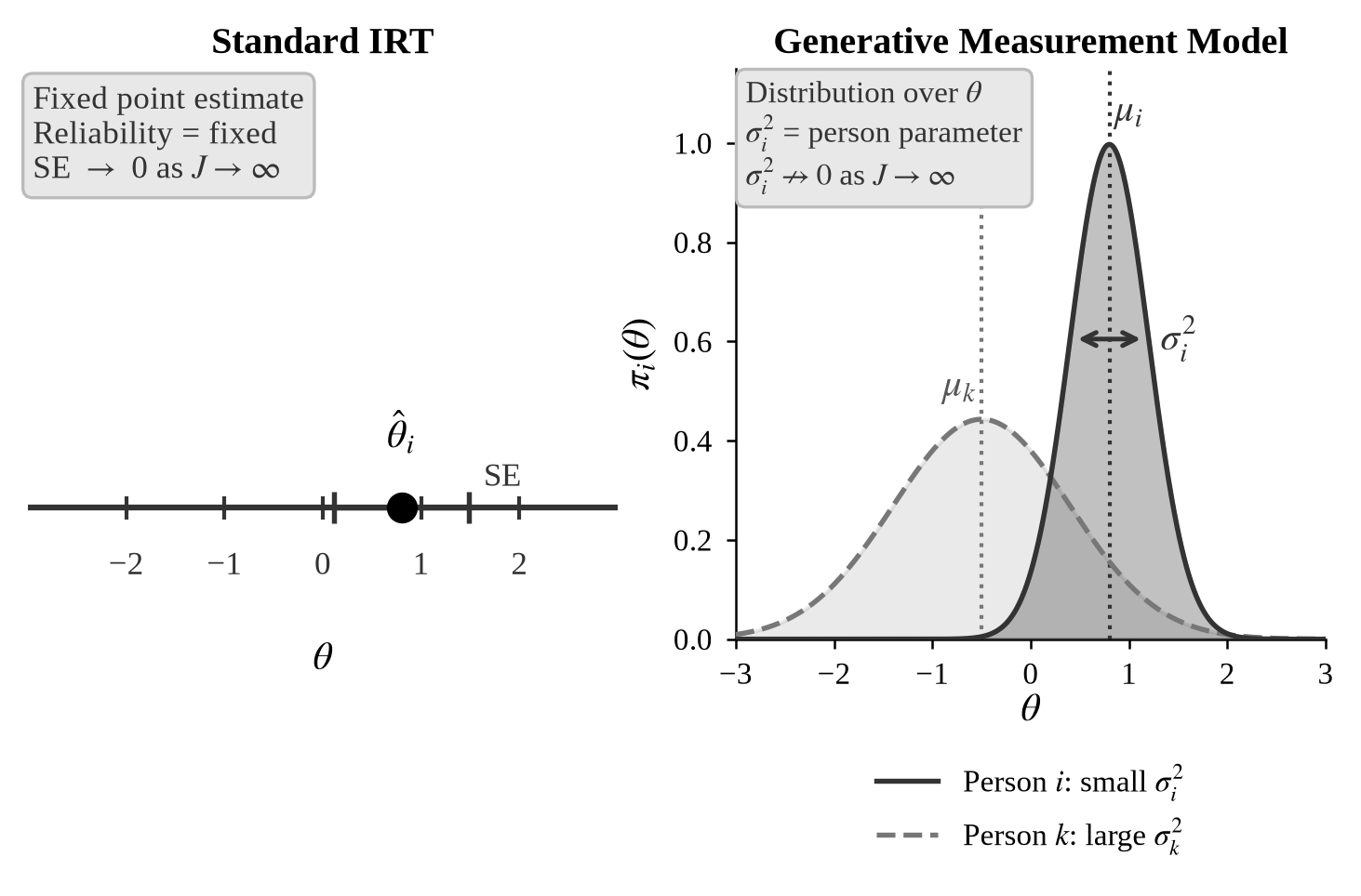
Figure 3. Standard IRT treats the person parameter as a fixed point with estimation error (left); the GMM treats it as a person-specific distribution with width as a substantive parameter (right). Under IRT, SE converges to zero with increasing items. Under GMM, distributional width is a stable person parameter that does not vanish with additional measurement.

2.6 Engagement with Existing Frameworks

The GMM relates to several established research programmes, and positioning it precisely relative to each is essential for evaluating what the framework adds. Fox (2010) develops an extensive Bayesian framework for IRT sharing Model A’s likelihood structure. The critical difference is that Fox’s person-specific prior represents population-level heterogeneity, whereas the GMM’s identity distribution represents within-person variability constituting a substantive individual difference in its own right. De Boeck, Cho & Wilson (2011) develop mixture IRT models capturing population heterogeneity, whereas the GMM captures within-person distributional variability. van Rijn, Dolan & Molenaar (2010) develop state-space models for IRT in which a latent trait evolves over time. The formal structure shares the ambition of modelling dynamic latent traits, but measurement and transition equations remain separate in that framework, whereas the GMM couples them. Borsboom & Cramer (2013) propose the network approach, operating at a different level of analysis. The two are not necessarily incompatible.

Fleeson & Jayawickreme (2015) articulate Whole Trait Theory, which reconceptualises personality traits as density distributions of states. The GMM provides what is, to the present author’s knowledge, the first measurement-theoretic formalisation of WTT’s distributional insight. WTT describes the phenomenon of personality as distribution but does not develop a psychometric model for estimating distributional parameters from item response data. The GMM’s identity distribution is the formal counterpart of WTT’s density distribution, and the GMM goes beyond WTT in embedding the distributional representation within a likelihood-based estimation framework and introducing the state transition mechanism.

Steyer, Schmitt & Eid (1999) develop latent state-trait theory, which decomposes observed score variance into trait, state, and measurement error. LST theory shares the GMM’s recognition that responses reflect both stable and occasion-specific components, but treats state variance as nuisance. The GMM reframes state variance as a substantive person parameter, as two people with the same trait mean but different state variances are psychologically different in a way that LST theory acknowledges descriptively but does not exploit psychometrically. Wu et al. (2024) and Kloft et al. (2023) represent concurrent developments that share aspects of the GMM’s distributional ambition, in that Wu et al. propose an individual random effects model incorporating within-person variance as a scale parameter, and Kloft et al. develop the Dirichlet dual response model for continuous bounded interval responses; both corroborate the distributional measurement programme from different starting points, although neither incorporates the measurement-as-intervention mechanism that constitutes the GMM’s distinctive contribution.

Ferrando’s programme on PDD warrants extended engagement, as it represents the most sustained effort within the IRT tradition to model person-level response variability as an individual-difference parameter. Ferrando (2016) introduces PDD within a dual model for binary personality responses, whereby each person carries a discrimination parameter alongside the standard trait level, and develops estimation and fit procedures through the InDisc framework (Ferrando & Navarro-González, 2020). Ferrando (2019) extends the approach to graded and continuous responses, and Ferrando & Navarro-González (2021) develop a multidimensional extension. The PDD programme partially anticipates the GMM’s distributional insight, and readers familiar with Ferrando’s work will rightly ask how ${\mathit{\sigma}_{\mathit{i}}}^{2}$ differs from PDD. The answer is fivefold. Firstly, PDD models person-level response variability as a nuisance parameter reflecting estimation uncertainty about a point trait level, so that the dispersion captures the imprecision with which the person’s fixed location is estimated from the item response process. The GMM treats ${\mathit{\sigma}_{\mathit{i}}}^{2}$ as ontological, in that the person is a distribution, and the width is a second measurand rather than error to be corrected. Secondly, PDD operates within the IRT framework as an extension, whereas the GMM subsumes IRT as a degenerate special case (Theorem 1), obtaining the standard 2PL when ${\mathit{\sigma}_{\mathit{i}}}^{2}$ approaches zero and $\mathit{w}_{\mathit{j}}$ equals zero. Thirdly, PDD does not incorporate measurement-as-intervention; the state transition equation coupling measurement to self-model revision through $\mathit{\kappa}_{\mathit{i}}$ and $\mathit{w}_{\mathit{j}}$ has no counterpart in Ferrando’s models. Fourthly, PDD does not include item identity-relevance weights ($\mathit{w}_{\mathit{j}}$), and therefore cannot generate the prediction that response variability should be concentrated on identity-relevant items rather than distributed uniformly. Lastly, PDD lacks the connection to predictive processing and self-model theory that grounds the GMM’s distributional claim in a computational account of why persons are distributions rather than points on self-reflective constructs. Nevertheless, Ferrando’s demonstration that person-level response variability can be reliably estimated within an IRT framework corroborates a prerequisite of the GMM programme, and the InDisc software provides existing infrastructure that future GMM implementations can build upon.

3. Distributional Reliability

3.1 Three Sources of Variability

Classical test theory partitions observed score variance into true score variance and error variance, a decomposition so foundational that it has structured psychometric thinking for over half a century (Lord & Novick, 1968). The GMM requires a different decomposition, one that recognises three distinct sources of response variability and assigns substantive meaning to two of them. The failure to distinguish these sources has, this section argues, produced a systematic misattribution of signal as noise in the measurement of self-reflective constructs.

The first source is between-person variance in posterior location parameters $\mathit{\mu}_{\mathit{i}}$, capturing stable individual differences in where each person’s self-model distribution is centred on the construct continuum. This component functions analogously to true score variance in classical theory.

The second source is within-person variance ${\mathit{\sigma}_{\mathit{i}}}^{2}$, the width of each individual’s identity distribution over self-model states. This component has no analogue in classical test theory because classical theory lacks the representational machinery to distinguish it from error. Under the GMM, ${\mathit{\sigma}_{\mathit{i}}}^{2}$ reflects the genuine breadth of an individual’s self-model on a given dimension, and it is a second measurand rather than noise. Critically, within-person variance is not placed in the denominator of any reliability coefficient under the GMM framework, because doing so would treat substantive signal as noise.

The third source is measurement error in the conventional sense: the residual stochasticity arising from the item response model that cannot be attributed to either between-person location differences or within-person distributional width. This is genuine noise, and it belongs in the denominator of the reliability coefficient.

The tripartite decomposition has immediate consequences for how instruments are evaluated. Fleeson (2001) demonstrates that within-person variability in behavioural states follows systematic, predictable distributions rather than random fluctuation around a fixed point, a finding that the GMM decomposition provides the formal apparatus to integrate into measurement theory (the first such integration, to the author’s knowledge, within a likelihood-based framework). Under classical test theory, an instrument that produces high within-person variability across occasions receives a low reliability coefficient, regardless of whether that variability is attributable to genuine distributional breadth or to measurement failure. Under the GMM decomposition, these two sources are formally separated.

The consequences extend to practical test development. An instrument optimised for classical reliability systematically selects against items that are sensitive to within-person distributional breadth, because such items contribute variability that classical reliability treats as error. Instruments refined through iterative item analysis under classical criteria will tend to converge on anchor items with high IRT discrimination and low sensitivity to ${\mathit{\sigma}_{\mathit{i}}}^{2}$. Items that would function as probe items, providing information about distributional width at the cost of increased response variability, are precisely the items that classical item analysis selects out.

3.2 GMM Reliability

The standard reliability coefficient under the GMM takes the form

$$\mathit{\rho}_{\text{GMM}}\ = \ {\mathit{\sigma}_{\text{between} - \mathit{\mu}}}^{2}\ /\ \left( {\mathit{\sigma}_{\text{between} - \mathit{\mu}}}^{2}\ + \ {\mathit{\sigma}_{\text{measurement}}}^{2} \right)$$

where ${\mathit{\sigma}_{\text{between} - \mathit{\mu}}}^{2}$ denotes the variance of posterior location parameters across persons and ${\mathit{\sigma}_{\text{measurement}}}^{2}$ denotes the variance attributable to the item response process after conditioning on both location and width parameters. The critical feature of this formulation is the exclusion of within-person variance ${\mathit{\sigma}_{\mathit{i}}}^{2}$ from the denominator. Classical reliability would place ${\mathit{\sigma}_{\mathit{i}}}^{2}$ in the denominator alongside ${\mathit{\sigma}_{\text{measurement}}}^{2}$, thereby inflating the apparent measurement error and distorting the reliability coefficient for any instrument administered to a sample containing persons with non-trivial distributional breadth.

A separate reliability coefficient is required for the second measurand, so that the precision of ${\mathit{\sigma}_{\mathit{i}}}^{2}$ estimation is evaluated independently of location estimation precision:

$$\mathit{\rho}_{\mathit{\sigma}}\ = \ {\mathit{\sigma}_{\text{between} - \mathit{\sigma ²}}}^{2}\ /\ \left( {\mathit{\sigma}_{\text{between} - \mathit{\sigma ²}}}^{2}\ + \ {\mathit{\sigma}_{\text{measurement} - \text{of} - \mathit{\sigma ²}}}^{2} \right)$$

An instrument might achieve high $\mathit{\rho}_{\text{GMM}}$ while achieving low $\mathit{\rho}_{\mathit{\sigma}}$, indicating successful location estimation but poor distributional recovery. The relationship between $\mathit{\rho}_{\text{GMM}}$ and classical reliability α is informative. Classical reliability conflates ${\mathit{\sigma}_{\text{between} - \mathit{\mu}}}^{2}$ and ${\mathit{\sigma}_{\mathit{i}}}^{2}$ in the numerator, and it places all variance except between-person true score variance in the denominator. The GMM decomposition reveals that classical reliability is a biased estimate of location measurement precision for instruments measuring self-reflective constructs, with the direction of bias depending on the ratio of within-person distributional variance to measurement error variance in the sample.

3.3 Distributional Precision

The paper proposes the Wasserstein-2 distance as the basis for a distributional precision metric. $\mathit{W}_{2}$ is a proper metric satisfying symmetry and the triangle inequality, is bounded for distributions on [0, 1], and has an intuitive interpretation as the minimum cost of transporting probability mass from one distribution to another. The distributional precision index takes the form

$$\mathit{W}\ = \ 1\ - \ \mathit{E}_{\mathit{i}}\left\lbrack \mathit{W}_{2}\left( {\widehat{\mathit{\pi}}}_{\mathit{i}},\ \mathit{\pi}_{\mathit{i}}^{\mathit{true}} \right) \right\rbrack\ /\ \mathit{W}_{\text{max}}$$

where the expectation is taken over persons and $\mathit{W}_{\text{max}}$ is calibrated against the maximum Wasserstein-2 distance between any two distributions on the construct’s support. This metric subsumes both location and width estimation quality, incentivising instrument development toward joint optimisation of location and distributional precision rather than the location-only optimisation that classical reliability promotes.

3.4 The ‘Unreliable Tests’ Hypothesis

The tripartite variance decomposition raises an uncomfortable possibility that must be stated with considerable care. If within-person variance constitutes genuine signal rather than noise, then instruments previously dismissed as unreliable might be capturing distributional information that classical reliability coefficients are structurally incapable of recognising. Not all unreliable tests are secretly measuring distributional width, and the claim is only that a specific, verifiable pattern of response variability would be expected if an instrument were capturing distributional information, and that this pattern can be distinguished from genuine measurement failure.

The distinction is empirically tractable. Distributional breadth, as it reflects a genuine property of the person’s self-model, should produce structured rather than random response variability. Three verification conditions must be satisfied before the distributional reinterpretation applies. Firstly, the metacognitive precision parameter $\mathit{\kappa}_{\mathit{i}}$ must be measured independently of the response data used to estimate distributional width, thereby preventing the circular attribution of response variability to a parameter estimated from that same variability. Secondly, within-occasion consistency must exceed between-occasion consistency for the instrument in question, a prediction that follows from the single-draw-per-occasion assumption and that genuine measurement failure does not predict. Thirdly, item-level variability should be concentrated on items with high estimated generative weight $\mathit{w}_{\mathit{j}}$ rather than uniformly distributed across all items. Genuinely unreliable measurement produces uniform variability, whereas distributional breadth produces variability concentrated on identity-relevant items. If all three conditions fail, the test is genuinely unreliable in the classical sense, and the distributional reinterpretation does not apply.

These verification conditions are specified with sufficient precision that the hypothesis is falsifiable, a requirement the clinical psychology literature rightly demands before any reinterpretation of established reliability findings. The hypothesis does not license a blanket reinterpretation of all test-retest inconsistency as distributional signal, and it must not be applied to clinical decision-making contexts without the specified verification procedures.

4. Items as Prediction-Error Generators

4.1 Generative Informativeness

Classical item analysis evaluates items by their discrimination and difficulty parameters, and the standard optimality criterion in adaptive testing (Fisher information) measures the expected curvature of the log-likelihood at a given trait level (van der Linden, 1998). Under the GMM, where the measurement target is an entire distribution characterised by the person parameter vector $\mathit{\psi}_{\mathit{i}}$ = ($\mathit{\mu}_{\mathit{i}}$, ${\mathit{\sigma}_{\mathit{i}}}^{2}$, $\mathit{\kappa}_{\mathit{i}}$), item evaluation requires a fundamentally different informativeness criterion that accounts for information about all distributional parameters simultaneously.

Generative informativeness for item j with respect to person i equals the expected information gain about the full distributional parameter vector

$$\mathit{I}_{\text{GMM}}\left( \mathit{j};\ \mathit{\psi}_{\mathit{i}} \right)\ = \ \mathit{E}_{\mathit{X}_{\mathit{ij}}}\left\lbrack KL\left( \mathit{p}\left( \mathit{\psi}_{\mathit{i}}\ |\ \mathit{x}_{\mathit{i},1:\mathit{j}} \right)\ \parallel \ \mathit{p}\left( \mathit{\psi}_{\mathit{i}}\ |\ \mathit{x}_{\mathit{i},1:\mathit{j} - 1} \right) \right) \right\rbrack$$

which amounts to the mutual information between the response $\mathit{X}_{\mathit{ij}}$ and the parameter vector $\mathit{\psi}_{\mathit{i}}$ given all previous responses. Under standard IRT, generative informativeness reduces to Fisher information evaluated at the point estimate ${\widehat{\mathit{\theta}}}_{\mathit{i}}$ when ${\mathit{\sigma}_{\mathit{i}}}^{2}$ = 0 and $\mathit{\kappa}_{\mathit{i}}$ is irrelevant, which establishes continuity with the existing adaptive testing framework.

The full computation is intractable for realistic assessment lengths. The paper proposes a Gaussian approximation to the consecutive posteriors, under which the KL divergence reduces to a tractable closed-form function of the change in mean vector and covariance matrix. The Gaussian approximation is adequate when the posteriors are approximately symmetric and unimodal, conditions satisfied after a sufficient number of items have been administered.

This formulation is related to the work of Tourangeau, Rips & Rasinski (2000), who propose a cognitive model of survey response, and of Embretson (1983, 1998), who develops construct representation. The GMM extends both by treating measurement reactivity as structural rather than artefactual, so that items with high $\mathit{w}_{\mathit{j}}$ engage the self-model more deeply and thereby generate more potential for self-model revision than items with low $\mathit{w}_{\mathit{j}}$.

4.2 Three-Type Item Taxonomy

The generative informativeness criterion motivates a design taxonomy that the paper presents as ideal-typical endpoints on a continuum of $\mathit{w}_{\mathit{j}}$ values rather than as rigid categories. Items in any instrument will fall along this continuum, and the taxonomy serves as a design framework for instrument construction under GMM rather than a classification scheme for existing items.

Anchor items occupy the low end of the $\mathit{w}_{\mathit{j}}$ continuum ($\mathit{w}_{\mathit{j}}$ ≈ 0), with clear meaning and high IRT discrimination. Under standard IRT, anchor items are simply good items. Under GMM, their primary contribution is location estimation, as they inform $\mathit{\mu}_{\mathit{i}}$ efficiently but provide little information about ${\mathit{\sigma}_{\mathit{i}}}^{2}$ or $\mathit{\kappa}_{\mathit{i}}$. Classical item analysis selects for anchor items by design, because the properties that make an item a good anchor are precisely the properties that classical item analysis rewards.

Probe items occupy the moderate range of the $\mathit{w}_{\mathit{j}}$ continuum, with content that admits multiple defensible readings and thereby engages self-reflective processing more deeply. Under standard IRT, probe items are problematic, exhibiting low discrimination and attenuated reliability. Under GMM, this interpretive variability makes probe items essential for width estimation, because the within-person response variability they produce is informative about ${\mathit{\sigma}_{\mathit{i}}}^{2}$ when the single-draw-per-occasion model holds.

Echo items serve a specialised diagnostic function, providing information about $\mathit{\kappa}_{\mathit{i}}$. An echo pair consists of two items with near-identical construct-relevant content presented at different points in the assessment. Under Model A, responses to both members should be highly consistent within an occasion. Within Model B, the consistency of echo pairs provides information about $\mathit{\kappa}_{\mathit{i}}$, as a respondent with high $\mathit{\kappa}_{\mathit{i}}$ will show systematic changes between pair members (reflecting within-occasion self-model updating) that a respondent with low $\mathit{\kappa}_{\mathit{i}}$ will not.

4.3 Adaptive Testing Under GMM

Adaptive testing under the GMM requires a multi-phase selection algorithm that differs qualitatively from standard computerised adaptive testing. Standard CAT selects items to maximise Fisher information at the current trait estimate, a criterion that concentrates items near the respondent’s estimated location and converges rapidly on a precise point estimate. GMM-based adaptive testing must balance three objectives simultaneously, as the algorithm must estimate $\mathit{\mu}_{\mathit{i}}$ and ${\mathit{\sigma}_{\mathit{i}}}^{2}$ and, if auxiliary data are being collected, $\mathit{\kappa}_{\mathit{i}}$.

The resulting algorithm proceeds in three phases. In the early phase, the algorithm preferentially selects anchor items, because the location estimate must be reasonably precise before width estimation becomes meaningful. As the location estimate stabilises, the algorithm transitions to a mixed strategy incorporating probe items whose generative informativeness for ${\mathit{\sigma}_{\mathit{i}}}^{2}$ exceeds a threshold. Throughout, echo items are interspersed at algorithmically determined intervals, with the spacing between echo pair members governed by the current estimate of $\mathit{\kappa}_{\mathit{i}}$ and the desired precision of that estimate.

The resulting assessment behaviour generates a testable prediction at the level of observable item selection patterns, in that GMM-based CAT should exhibit three distinguishing features compared with IRT-based CAT. Firstly, GMM-based CAT should select a broader range of item difficulties, because probe items at diverse locations provide information about distributional width that items concentrated near $\mathit{\mu}_{\mathit{i}}$ cannot. Secondly, GMM-based CAT should exhibit a characteristic temporal profile, transitioning from location-focused to width-focused item selection as the assessment progresses. Lastly, GMM-based CAT should produce adaptive assessments that vary more across persons in their item selection patterns, because the item selection criterion depends on the full parameter vector $\mathit{\psi}_{\mathit{i}}$ rather than the scalar ${\widehat{\mathit{\theta}}}_{\mathit{i}}$, and persons who differ in ${\mathit{\sigma}_{\mathit{i}}}^{2}$ or $\mathit{\kappa}_{\mathit{i}}$ will generate different item selection trajectories even when their $\mathit{\mu}_{\mathit{i}}$ values are identical.

5. The Replication Crisis – Formally

5.1 Test-Retest Predictions Under GMM

The GMM generates a structured set of predictions about test-retest reliability that are jointly more specific than any competing account can produce. The predictions of this section invoke $\mathit{\kappa}_{\mathit{i}}$, which requires auxiliary data for estimation (as Section 2.4 acknowledges). These predictions are therefore consequences of the full theoretical framework rather than of Model A alone, and their empirical test presupposes the identification strategies outlined in Section 2.4. Conditional on the availability of auxiliary data or Model B estimation, the following predictions obtain.

The first prediction concerns the three-way interaction among metacognitive precision $\mathit{\kappa}_{\mathit{i}}$, posterior width ${\mathit{\sigma}_{\mathit{i}}}^{2}$, and generative weight $\mathit{w}_{\mathit{j}}$. The interaction takes the following form. A person with narrow posterior (low ${\mathit{\sigma}_{\mathit{i}}}^{2}$) and high $\mathit{\kappa}_{\mathit{i}}$ shows high retest reliability, because measurement generates negligible prediction error against a precise self-representation. The self-model is sufficiently crystallised that item-generated perturbations produce minimal updating, regardless of the person’s metacognitive transparency. A person with broad posterior (high ${\mathit{\sigma}_{\mathit{i}}}^{2}$) and high $\mathit{\kappa}_{\mathit{i}}$ shows low retest reliability, because they are accurately sampling from a genuinely variable self-model on each occasion, and their high metacognitive precision ensures that the prediction errors generated by measurement produce non-trivial self-model updates. A person with low $\mathit{\kappa}_{\mathit{i}}$, regardless of posterior width, shows moderate retest reliability, because their metacognitive opacity produces a cached point estimate partially insensitive to the identity distribution’s actual breadth. They report roughly the same value on each occasion not because their distribution is narrow but because their self-model querying process is imprecise.

The second prediction concerns item identity-relevance. High-$\mathit{w}_{\mathit{j}}$ items should show more retest instability than low-$\mathit{w}_{\mathit{j}}$ items, and this difference should be modulated by $\mathit{\kappa}_{\mathit{i}}$. Factual knowledge items ($\mathit{w}_{\mathit{j}}$ ≈ 0) should show standard stability regardless of $\mathit{\kappa}_{\mathit{i}}$ or ${\mathit{\sigma}_{\mathit{i}}}^{2}$. Identity-statement items (high $\mathit{w}_{\mathit{j}}$) should show maximum instability for high-$\mathit{\kappa}_{\mathit{i}}$ respondents with broad posteriors. This item-level specificity distinguishes GMM from generic instability explanations.

The third prediction concerns parallel-form reliability. For high-$\mathit{\kappa}_{\mathit{i}}$ people on broad-posterior dimensions, same-form retest includes a memory component that partially compensates for distributional sampling variability. Parallel forms eliminate this compensation, producing lower reliability than same-form for high-$\mathit{\kappa}_{\mathit{i}}$ respondents, which reverses the classical expectation.

The main effect of distributional width on retest variability, as indexed by the cross-factor variance proxy of Section 2.4, is empirically robust (beta positive in eight of nine tests, d = 0.55; Morrison, 2026g), confirming that persons with wider identity distributions produce more variable retest responses, as the framework predicts. Item-level analysis (N = 1,030 retest pairs, 50 items; Morrison, 2026g) reveals that the $\mathit{\kappa}_{\mathit{i}}$ × $\mathit{w}_{\mathit{j}}$ interaction is statistically significant in multilevel modelling (β = −0.031, p = .013) but in the wrong direction, as high-$\mathit{\kappa}_{\mathit{i}}$ individuals show less retest instability on high-identity-relevance items, not more. The main effect of the same proxy on overall variability is robust at item level (β = 0.186, p < 10⁻¹⁰, positive for all 50 items), confirming that persons high on it are more variable overall. This conjunction of greater global variability and selective stability on identity-relevant items is consistent with precision-as-investment (Section 2.2) rather than precision-as-update-rate. The original prediction that the $\mathit{\kappa}_{\mathit{i}}$ × $\mathit{w}_{\mathit{j}}$ interaction would be positive assumed that metacognitive precision functions as a uniform update rate, such that high-$\mathit{\kappa}_{\mathit{i}}$ individuals revise their self-models more extensively on identity-relevant items. The empirical finding indicates instead that high-$\mathit{\kappa}_{\mathit{i}}$ individuals selectively protect identity-relevant items from perturbation, investing precision resources precisely where self-model integrity is most at stake. The framework’s core claim (that distributional width and metacognitive precision jointly determine retest variability) is preserved, although the direction of the interaction requires the revised interpretation of $\mathit{\kappa}_{\mathit{i}}$ developed in Section 2.2.

5.2 Reconciliation with Big Five Stability

The foregoing predictions must be reconciled with the most robust finding in personality measurement – the demonstration by Roberts & DelVecchio (2000) that rank-order stability of Big Five traits reaches r > .70 by age 50 and remains at that level or higher thereafter. The GMM framework not only accommodates this finding but derives it as a consequence of posterior narrowing with age.

The predicted test-retest correlation under GMM takes the form

$$\mathit{r}_{\mathit{tt}}\ \approx \ {\mathit{\sigma}_{\text{between} - \mathit{\mu}}}^{2}\ /\ \left( {\mathit{\sigma}_{\text{between} - \mathit{\mu}}}^{2}\ + \ \mathit{g}\left( \mathit{\kappa},\ \mathit{\sigma ²},\ \mathit{w} \right)\ + \ {\mathit{\sigma}_{\text{error}}}^{2} \right)$$

where g(κ, $\mathit{\sigma ²}$, w) represents the contribution of measurement-reactive distributional variability – a function of the sample’s distribution of $\mathit{\kappa}_{\mathit{i}}$ values, ${\mathit{\sigma}_{\mathit{i}}}^{2}$ values, and the instrument’s $\mathit{w}_{\mathit{j}}$ profile. When ${\mathit{\sigma}_{\mathit{i}}}^{2}$ is small for the majority of respondents, g approaches zero, and $\mathit{r}_{\mathit{tt}}$ approaches classical reliability. The Roberts & DelVecchio age-stability trajectory emerges as a direct consequence of a developmental process in which the identity distribution narrows with accumulating experience. Decades of identity-relevant experience provide a massive evidence base against which new prediction errors are evaluated, and the resulting posterior precision renders the self-model increasingly resistant to perturbation by any single measurement occasion. The developmental trajectory predicted by GMM is monotonic narrowing of ${\mathit{\sigma}_{\mathit{i}}}^{2}$ with age for the majority of people on the majority of Big Five dimensions, producing the increasing rank-order stability that Roberts & DelVecchio document.

This reconciliation generates a subsidiary prediction. Rank-order stability should be lower for dimensions on which the population exhibits high ${\mathit{\sigma}_{\mathit{i}}}^{2}$, and should increase more slowly with age for dimensions on which identity crystallisation is slower. If extraversion crystallises earlier than openness, the age-stability trajectory should show earlier plateau for extraversion. This is a novel prediction that standard IRT cannot generate, as it does not represent distributional width. Costa & McCrae (1992) provide normative data on differential trait stability that could be re-examined on this basis.

5.3 The Paradoxical Prediction

The most striking prediction of the GMM framework is that the most metacognitively accurate people should show the lowest naive test-retest reliability on broad-posterior dimensions. This prediction is paradoxical in the precise sense that it reverses the intuitive expectation that more self-aware people should be more consistent reporters. Under the GMM, high-$\mathit{\kappa}_{\mathit{i}}$ people are indeed more accurate reporters, accurately tracking a genuinely variable self-model rather than producing a cached point estimate. Their apparent inconsistency is therefore a matter of fidelity to the self-model, and does not indicate failure.

Three conditions must be jointly satisfied before this interpretation applies, and the paper specifies these conditions to prevent the paradoxical prediction from being applied as a blanket reinterpretation of all test-retest inconsistency. Firstly, the variability must be structured rather than random, concentrated on specific items and following a pattern consistent with the single-draw-per-occasion model. Secondly, the variability must be concentrated on high-$\mathit{w}_{\mathit{j}}$ items rather than uniformly distributed across the assessment; genuinely poor measurement produces uniform inconsistency, whereas distributional sampling produces item-specific inconsistency. Lastly, the respondent must have independently measured $\mathit{\kappa}_{\mathit{i}}$ in the upper range. Without independent measurement of metacognitive precision, the attribution of inconsistency to accurate distributional sampling rather than to measurement failure is empirically underdetermined. Without all three conditions, low retest reliability means what it has always meant within the classical framework.

6. Empirical Programme

6.1 Study 1: Parameter Recovery Simulation

The first study evaluates whether the distributional parameters of Model A can be recovered from simulated data under conditions representative of realistic personality assessment. The full design, which has not yet been run, generates data from N = 1,000 simulated persons responding to assessment items under three test-length conditions (J = 30, 50, and 100 items) across T = 5 measurement occasions. Person parameters are drawn such that $\mathit{\mu}_{\mathit{i}}$ is sampled from Uniform(−2, 2), $\mathit{\sigma}_{\mathit{i}}$ from Uniform(0.3, 1.5), and $\mathit{\kappa}_{\mathit{i}}$ from Beta(3, 3). The identity distribution is modelled as Gaussian N($\mathit{\mu}_{\mathit{i}}$, ${\mathit{\sigma}_{\mathit{i}}}^{2}$). Item parameters follow the 2PL structure with $\mathit{a}_{\mathit{j}}$ from LogNormal(0, 0.5), $\mathit{b}_{\mathit{j}}$ from Normal(0, 1), and $\mathit{w}_{\mathit{j}}$ from Beta(2, 5), producing a right-skewed distribution of identity-relevance weights with most items having low to moderate $\mathit{w}_{\mathit{j}}$.

Data generation under Model A proceeds by the single-draw mechanism. For each person on each occasion, $\mathit{\theta}_{\mathit{it}}^{\mathit{\ast}}$ is drawn from N($\mathit{\mu}_{\mathit{i}}$, ${\mathit{\sigma}_{\mathit{i}}}^{2}$), and binary item responses are generated independently conditional on this draw according to the 2PL item response function. This generation process guarantees that the true distributional parameters are known and that the simulation provides a fair test of the estimation procedure.

Estimation in the full design employs data augmentation MCMC with three sampling steps: (1) sample $\mathit{\theta}_{\mathit{it}}^{\mathit{\ast}}$ from its full conditional via Metropolis-Hastings with a normal proposal, (2) sample ($\mathit{\mu}_{\mathit{i}}$, ${\mathit{\sigma}_{\mathit{i}}}^{2}$) via conjugate normal-inverse-gamma updates given the sampled $\mathit{\theta}_{\mathit{it}}^{\mathit{\ast}}$ values across occasions, and (3) sample item parameters ($\mathit{a}_{\mathit{j}}$, $\mathit{b}_{\mathit{j}}$) via standard 2PL Bayesian procedures conditional on all sampled $\mathit{\theta}_{\mathit{it}}^{\mathit{\ast}}$ values. Four chains are run for 15,000 iterations each with 5,000 warmup iterations. Convergence is assessed via R-hat < 1.01, bulk ESS > 400, and tail ESS > 400 for all monitored parameters.

Three scenarios evaluate the contribution of different data sources to parameter recovery: (a) response data only, with the estimation relying entirely on the multi-occasion response patterns; (b) response data with 10 echo pairs interspersed in the instrument, providing within-occasion information about response consistency beyond what the standard items provide; and (c) response data plus response times under a joint LogNormal response time model, in which response time is modelled as a function of item time-intensity, person speed, and an interaction between ${\mathit{\sigma}_{\mathit{i}}}^{2}$ and item difficulty predicted to produce flatter response time gradients for broad-posterior persons.

Performance metrics include bias (mean difference between estimated and true parameter values), root mean squared error (RMSE), Pearson correlation between estimated and true values, and coverage of 95% posterior credible intervals. These metrics are computed separately for $\mathit{\mu}_{\mathit{i}}$, ${\mathit{\sigma}_{\mathit{i}}}^{2}$, and, in Scenarios (b) and (c), $\mathit{\kappa}_{\mathit{i}}$.

A priori benchmarks are specified to discipline the interpretation of results. ${\mathit{\sigma}_{\mathit{i}}}^{2}$ recovery is considered adequate if the correlation between estimated and true values exceeds 0.6 and the relative RMSE (RMSE divided by the standard deviation of true values) falls below 0.5. $\mathit{\kappa}_{\mathit{i}}$ recovery is considered adequate if the correlation between estimated and true values exceeds 0.5, a less stringent criterion reflecting the greater difficulty of identifying this parameter. If ${\mathit{\sigma}_{\mathit{i}}}^{2}$ recovery fails these benchmarks at J = 100 items under all three scenarios, the paper will conclude that distributional measurement is impractical for individual-level assessment and that the framework’s contribution is theoretical rather than empirical.

A preliminary simulation under Scenario (a), response data only, with N = 500 persons, T = 5 occasions, and item parameters fixed at their generating values, yields the following results from one replicate per condition. It ran four chains of 5,000 iterations with 2,000 warmup, under the priors $\mathit{\mu}_{\mathit{i}}$ ~ N(0, 4) and ${\mathit{\sigma}_{\mathit{i}}}^{2}$ ~ IG(2, 1), whose mean of 1.0 sits beside a true population mean of .93, with separate normal and inverse-gamma conditional updates. Unsplit R-hat reached 1.014 for ${\mathit{\sigma}_{\mathit{i}}}^{2}$ at J = 30, above the 1.01 criterion, and ESS was not computed. Scenarios (b) and (c) have not yet been run.

For $\mathit{\mu}_{\mathit{i}}$ recovery, correlation with true values is .93 to .94 across all test lengths (J = 30, 50, 100), with bias below .04, relative RMSE below .40, and 95% credible interval coverage at .94–.95 – comparable to standard IRT θ estimation. For ${\mathit{\sigma}_{\mathit{i}}}^{2}$ recovery under the same conditions, correlation with true values reaches .52 at J = 30, .55 at J = 50, and .60 at J = 100, with relative RMSE of 1.09, .99 and .92, bias of .08, .05 and .05, and 95% coverage of .89, .88 and .89. A relative RMSE of 1.0 is what reporting the population mean for everyone achieves. Cross-correlations between true μ and estimated $\mathit{\sigma ²}$, and between true $\mathit{\sigma ²}$ and estimated μ, are near zero (|r| < .07), confirming that the two parameters are not confounded in estimation. A supplementary analysis with T = 10 occasions at J = 100 items raises the ${\mathit{\sigma}_{\mathit{i}}}^{2}$ correlation to .73, with relative RMSE .80 and coverage .91, demonstrating that the number of measurement occasions is the primary determinant of distributional parameter recovery. These results indicate that ${\mathit{\sigma}_{\mathit{i}}}^{2}$ is identifiable and that its recovery improves monotonically with both test length and number of occasions, although every condition run falls below the benchmark above, since r reaches only .60 at T = 5, on one replicate, and relative RMSE stays at .80 or above.

The shortfall lies in the number of occasions and not in the number of items. With $\mathit{\theta}_{\mathit{it}}^{\mathit{\ast}}$ known exactly, as under unbounded J, the study’s prior gives relative RMSE of .90 at T = 5, .71 at T = 10, .53 at T = 20 and .39 at T = 40, and the true population distribution of $\mathit{\sigma}_{\mathit{i}}$, used as the prior, gives .70 at T = 5, .55 at T = 10 and .47 at T = 15, so no test length clears the benchmark at the T = 5 of the design or at T = 10, and clearing it takes roughly fifteen occasions at best and more than twenty under the study’s prior. The framework’s primary empirical utility at current precision levels is expected to pertain to group-level comparisons and longitudinal tracking rather than individual-level distributional classification, an expectation no group comparison or power analysis has yet tested.

6.2 Study 2: Re-Analysis of Existing Test-Retest Data

The second study applies the GMM to existing test-retest data to test whether distributional parameters improve prediction of retest responses beyond what standard IRT provides. The target dataset is the Eugene-Springfield Community Sample (Goldberg, 1999), a longitudinal study of approximately 800 community volunteers who completed item-level personality inventories, including the 240-item NEO PI-R, across multiple waves spanning over a decade, with item-level data publicly available on Harvard Dataverse. A secondary dataset is the HEXACO-PI-R test-retest dataset (Henry et al., 2022), which provides N = 416 participants completing 100 items on two occasions separated by a median of 13 days, with data publicly available on OSF.

The analysis proceeds as follows. Firstly, standard 2PL IRT and Model A GMM are both fitted to occasion-1 data. Secondly, both models are used to predict occasion-2 item-level responses. Predictive accuracy is compared via leave-one-out cross-validation (LOO-CV) or widely applicable information criterion (WAIC; Watanabe, 2010; Vehtari, Gelman & Gabry, 2017), both of which account for parameter count and thereby penalise the GMM’s additional parameters.

The critical test goes beyond aggregate model comparison. The analysis regresses retest variability, defined as the within-person standard deviation of occasion-2 residuals from the IRT model, on the GMM’s estimated ${{\widehat{\mathit{\sigma}}}_{\mathit{i}}}^{2}$ from occasion-1, controlling for the IRT point estimate ${\widehat{\mathit{\theta}}}_{\mathit{i}}$, the IRT standard error (which captures estimation uncertainty under the point-estimate model), and person-fit statistics (Meijer & Sijtsma, 2001) that capture aberrant response patterns without a metacognitive interpretation. If ${{\widehat{\mathit{\sigma}}}_{\mathit{i}}}^{2}$ explains incremental variance in retest variability beyond these controls, the distributional extension has demonstrated empirical value. If it does not, the additional parameters have not justified their inclusion, and the framework’s contribution remains theoretical.

6.3 Proposed Experimental Studies

Three experimental studies are proposed as future work to test the predictions that the simulation and re-analysis studies cannot address.

Study 3 (κ moderation): N = 400, 2 × 2 design (high/low $\mathit{\kappa}_{\mathit{i}}$ × short/long retest interval). Participants complete a metacognitive calibration task and a 50-item personality measure at Session 1, with Session 2 (retest) at either one week or one month. The GMM predicts a $\mathit{\kappa}_{\mathit{i}}$ × interval interaction on reliability, such that high-$\mathit{\kappa}_{\mathit{i}}$ participants show greater reliability decline across the longer interval. Falsification criterion: a non-negative regression coefficient for $\mathit{\kappa}_{\mathit{i}}$ ($\mathit{\beta}_{1}$ ≥ 0) indicates the metacognitive channel is not operating as theorised.

Study 4 (within versus between consistency): N = 300, 60 items, 20 repeated within-session. This study directly tests the single-draw prediction by comparing within-occasion consistency to between-occasion consistency on the same items. Falsification criterion: between-occasion consistency exceeding within-occasion consistency after controlling for memory effects would refute the single-draw model.

Study 5 (item-type sensitivity): N = 500, 90 items (30 anchors, 30 probes, 30 echoes). This study tests whether the item taxonomy translates into differential information provision for distributional parameters. Falsification criterion: probe items uninformative about ${\mathit{\sigma}_{\mathit{i}}}^{2}$ under GMM would indicate the item-as-prediction-error-generator theory does not generate the expected design implications.

7. Trajectory Validity and the Measurement-as-Intervention Problem

The preceding sections have developed a measurement framework in which the act of measurement can alter the measurand, distributional parameters constitute person-level estimands, and metacognitive precision moderates the relationship between measurement and self-model revision. These claims create a fundamental tension with the dominant philosophical account of construct validity, a concept whose modern formulation originates with Cronbach & Meehl (1955). The present section argues that resolving this tension requires not the abandonment of validity as a regulative concept but its reconceptualisation for the class of constructs where the passivity assumption fails.

7.1 The Construct Validity Paradox

Borsboom, Mellenbergh & van Heerden (2004) advance a realist-causal account of construct validity according to which a test is valid if and only if variation in the attribute causally produces variation in test scores. The account presupposes that the attribute exists independently of the measurement procedure, and that the causal arrow runs from attribute to score without a return path through which measurement modifies the attribute. For ability constructs, this presupposition holds to a reasonable approximation.

For self-reflective constructs, the GMM predicts that this presupposition fails. When an item functions as a prediction-error generator with non-zero identity-relevance ($\mathit{w}_{\mathit{j}}$ > 0), responding updates the respondent’s self-model distribution. This generates three problems for Borsboom’s account. Firstly, test-retest reliability becomes conceptually incoherent, given that the second measurement assesses an attribute the first measurement helped to constitute. Secondly, convergent validity is undermined in its classical formulation (Campbell & Fiske, 1959), as two valid measures may produce different posterior updates precisely because they present different prediction errors. Lastly, the construct becomes partially instrument-dependent.

7.2 Trajectory Validity

The resolution proposed here reconceives validity for self-reflective constructs as trajectory validity. Where Borsboom’s account defines validity in terms of the causal relationship between a fixed attribute and an indicator, trajectory validity defines it in terms of the dynamical relationship between a measurement procedure and the trajectory of the self-model through parameter space.

The formal intuition proceeds as follows. A self-reflective construct corresponds not to a fixed point in parameter space but to a basin of attraction (a region of the distributional parameter space within which the self-model tends to remain under ordinary experience and self-reflection). A measurement procedure is trajectory-valid when the prediction errors it generates move the respondent’s self-model within the appropriate basin rather than displacing it into an adjacent basin. More precisely, a test with items {j} is trajectory-valid for construct C if the posterior distribution $\mathit{\pi}_{\mathit{i}}^{\left( \mathit{J} \right)}$(θ), obtained after the respondent has processed all J items, remains within the basin corresponding to C in the construct’s theoretical network.

This reconceptualisation preserves the normative force of validity. There remain right and wrong ways to measure conscientiousness. A measure that induces the respondent to revise their self-model in directions inconsistent with the construct’s theoretical network is invalid regardless of how much information it provides about distributional parameters. Trajectory validity is thus a genuine validity concept, not an abandonment of validity, although it is one that accepts the constitutive role of measurement in the domain where that role operates.

7.3 Convergent Validity Under Measurement-as-Intervention

The trajectory validity framework reinterprets convergent validity for self-reflective constructs. Campbell & Fiske (1959) define convergent validity as agreement between different methods measuring the same trait. Under the trajectory validity account, convergent validity requires that two valid measures generate trajectories within the same basin of attraction, although those trajectories may differ in their specific path through the basin. Convergent validity is thus reframed as basin convergence rather than point convergence. Where basins overlap, as they plausibly do for closely related constructs, trajectory validity predicts that discriminant validity will be more difficult to establish for self-reflective constructs than for ability constructs – a prediction consistent with the well-documented difficulty of achieving clean discriminant validity in personality measurement.

7.4 Connection to Reactive Measurement and Latent State-Trait Theory

Webb, Campbell, Schwartz & Sechrest (1966) documented the problem of reactive measurement decades before the present framework provided formal tools for its analysis. The trajectory validity concept formalises what the unobtrusive measures tradition described informally. Steyer, Schmitt & Eid (1999) develop Latent State-Trait theory, which treats state variability as nuisance variance, whereas the GMM framework treats it as potentially informative about distributional parameters. The trajectory validity concept accommodates both accounts as special cases, with LST theory applying when distributional breadth is negligible.

7.5 When Trajectory Validity Reduces to Classical Validity

For ability constructs, where $\mathit{w}_{\mathit{j}}$ approaches 0, measurement does not perturb the self-model. The basin of attraction collapses to a single fixed point, and trajectory validity reduces to Borsboom’s standard realist-causal account. The GMM’s validity concept is therefore a generalisation of the classical concept and does not replace it.

Michell (2000, 2008) argues that psychometrics assumes without justification that psychological attributes are continuous quantities. The distributional measurand of GMM responds to this critique directly, as it constitutes a different kind of quantitative structure characterised by shape parameters rather than point magnitudes. Whether shape parameters satisfy the conditions for genuine quantitative measurement is an empirical question the framework makes tractable rather than assumes away.

8. Objections and Responses

The preceding sections have advanced claims requiring defence from multiple directions simultaneously, and a paper proposing a new measurement theory for an important class of psychological constructs invites objections concerning its novelty, identifiability, empirical standing, and distributional assumptions. The present section addresses five objections, each stated in its strongest available formulation before a response is offered. A measurement theory paper must demonstrate that its formal apparatus justifies its additional complexity, and several of the objections below challenge precisely this.

8.1 ‘This Is Just a Random Effects Model’

The objection holds that the GMM likelihood is structurally identical to random-effects IRT (Fox, 2010) and that the paper relabels epistemological uncertainty as ‘ontological distributional breadth’ without adding predictive content. The charge is particularly damaging because Model A’s static likelihood is formally a marginal IRT model with a person-specific mixing distribution.

The response concedes the structural similarity whilst identifying three distinguishing features. Firstly, the state transition equation (through which measurement at occasion t feeds into the self-model distribution at occasion t + 1) is absent from random-effects IRT and generates a discriminating prediction. Under random-effects IRT, item order is irrelevant to the marginal likelihood. Under GMM with non-zero $\mathit{\kappa}_{\mathit{i}}$ and $\mathit{w}_{\mathit{j}}$, item order matters, because earlier items generate prediction errors that update the self-model distribution from which later responses are drawn.

Secondly, $\mathit{\kappa}_{\mathit{i}}$ is not merely a random effect but a theoretically motivated metacognitive parameter with independent empirical anchors, including metacognitive calibration tasks (Fleming & Lau, 2014) and private self-consciousness (Fenigstein, Scheier & Buss, 1975). Whether $\mathit{\kappa}_{\mathit{i}}$ correlates with independently measured metacognitive accuracy is an empirical question (Study 3, Section 6). The prediction exists and random-effects IRT does not generate it.

Lastly, the coupling between measurement and transition equations distinguishes GMM from dynamic measurement models (van Rijn, Dolan & Molenaar, 2010) in which these equations operate independently. GMM’s distinctive property is that responses generated through the measurement equation update the latent state through the transition equation, a coupling absent from all existing dynamic measurement models of which the author is aware.

8.2 ‘Identifiability Not Established’

The objection holds that ${\mathit{\sigma}_{\mathit{i}}}^{2}$ and $\mathit{\kappa}_{\mathit{i}}$ may not be jointly identifiable from single-occasion response data, because both parameters produce response variability and the product $\mathit{\kappa}_{\mathit{i}}$ · $\mathit{w}_{\mathit{j}}$ enters the likelihood rather than the individual components. This is the most serious threat to the framework’s practical utility.

The response is stratified. Model A recovers ${\mathit{\sigma}_{\mathit{i}}}^{2}$ from the between-occasion spread of the $\mathit{\theta}_{\mathit{it}}^{\mathit{\ast}}$ (Section 2.4), and the single-occasion route through the within-occasion correlation structure, in which a single draw from $\mathit{\pi}_{\mathit{i}}$(θ) generates all within-occasion responses and produces intercorrelations among items near the respondent’s location that exceed IRT predictions, remains conjectural (Conjecture 1). A rerun at J = 100 gives r = .12 at T = 1, .36 at T = 2 and .50 at T = 3, on one replicate each, and the .60 at T = 5 sits against .62 from between-occasion spread alone with $\mathit{\theta}_{\mathit{it}}^{\mathit{\ast}}$ known exactly. The preliminary simulation of Section 6.1 shows ${\mathit{\sigma}_{\mathit{i}}}^{2}$ to be identifiable but below the paper’s benchmark for adequate recovery under response data alone in every condition run (at J = 100, r = .60 with relative RMSE .92 at T = 5 and r = .73 with relative RMSE .80 at T = 10, against a required r above 0.6 and a required relative RMSE below 0.5), with Scenarios (b) and (c) not yet run. The identification of $\mathit{\kappa}_{\mathit{i}}$ from response data alone is an open problem, and the paper’s position is that $\mathit{\kappa}_{\mathit{i}}$ requires auxiliary data (echo items, response times, or external metacognitive calibration) for reliable estimation. The paper’s primary empirical contribution is distributional measurement, and $\mathit{\kappa}_{\mathit{i}}$ estimation remains a frontier, a limitation that leaves the distributional contribution intact.

8.3 ‘The Replication Crisis Explanation Is Post Hoc’

The objection holds that GMM’s explanation of the replication crisis is post hoc, and that any sufficiently flexible model can accommodate known results.

The response concedes the post hoc character and identifies the specificity of GMM’s predictions as the discriminating feature. GMM predicts a specific $\mathit{\kappa}_{\mathit{i}}$-by-$\mathit{w}_{\mathit{j}}$ interaction pattern in which instability is concentrated on high-identity-relevance items for high-$\mathit{\kappa}_{\mathit{i}}$ individuals. Practice effects predict uniform improvement across items. Mood effects predict mood-correlated shifts without item-specific moderation. Regression to the mean predicts moderation of extreme scores without κ-dependent patterns. Response style fluctuation predicts person-level variability without the item-specific pattern. The $\mathit{\kappa}_{\mathit{i}}$-by-$\mathit{w}_{\mathit{j}}$ interaction is not predicted by any competing account, and its presence or absence in test-retest data amounts to a discriminating test.

8.4 ‘κ Is Unfalsifiable’

The objection holds that $\mathit{\kappa}_{\mathit{i}}$ absorbs unexplained variance and cannot be independently constrained.

The response specifies falsification conditions explicitly. $\mathit{\kappa}_{\mathit{i}}$ must be measured independently through metacognitive calibration tasks (Fleming & Lau, 2014), private self-consciousness scales (Fenigstein, Scheier & Buss, 1975), or perceptual metacognition paradigms, and then used to predict test-retest instability above and beyond person-fit indices (Meijer & Sijtsma, 2001), response style measures (Wetzel, Lüdtke, Zettler & Böhnke, 2016), conscientiousness, and cognitive ability. If independently measured $\mathit{\kappa}_{\mathit{i}}$ does not predict the specific $\mathit{w}_{\mathit{j}}$-moderated pattern of item-level instability, the GMM-specific claim that $\mathit{\kappa}_{\mathit{i}}$ moderates measurement-as-intervention is unfounded. The parameter is falsifiable precisely because it generates predictions more specific than ‘people differ in response consistency.’

8.5 ‘The Beta Distribution Assumption Is Arbitrary’

The objection holds that the Beta distribution choice is a convenience assumption without theoretical justification.

The response distinguishes the distributional family from the distributional measurand claim. GMM depends on the claim that the measurand is a distribution rather than a point, not on any particular distributional family. The framework accommodates Gaussian (unbounded continua), Beta (bounded traits, with Gaussian/Beta reconciliation in which large total evidence produces convergence to Gaussian form; see Morrison, 2026b), and nonparametric (Dirichlet process) alternatives. The paper’s claims about distributional measurement, measurement-as-intervention, and the item taxonomy are invariant to the choice of family. The theoretical architecture is distribution-agnostic, whereas the implementation is distribution-specific.

9. Discussion and Conclusion

9.1 Summary of Contributions

The paper has developed a measurement theory for the class of psychological constructs where the passivity assumption fails (constructs for which the act of measurement can alter the attribute being measured). Three contributions have been advanced, each carrying commitments the empirical programme of Section 6 is designed to test.

The first contribution is the formal incorporation of measurement-as-intervention into the measurement model’s structural equations, in that the state transition equation couples measurement and state change in a manner absent from dynamic measurement models (van Rijn, Dolan & Molenaar, 2010), Bayesian adaptive testing (van der Linden, 1998), and network psychometrics (Borsboom & Cramer, 2013). The novelty pertains not to the discovery of reactivity (a phenomenon documented since Webb, Campbell, Schwartz & Sechrest (1966)) but to the formal machinery through which reactive measurement is incorporated into the model’s likelihood function and transition dynamics.

The second contribution is distributional measurement, in which ${\mathit{\sigma}_{\mathit{i}}}^{2}$ is estimated as a person parameter rather than discarded as measurement error. The distributional reliability framework of Section 3 implies that some instruments dismissed as unreliable may be capturing genuine distributional signal – a testable hypothesis (Section 6, Study 2) rather than a blanket reinterpretation of all test-retest inconsistency.

The third contribution is $\mathit{\kappa}_{\mathit{i}}$ as a continuous metacognitive precision parameter, which is theoretically novel although it requires auxiliary data for identification. If independently measured $\mathit{\kappa}_{\mathit{i}}$ does not predict the specific patterns GMM specifies, the framework’s contribution reduces to distributional measurement without the metacognitive channel.

The cumulative empirical record strengthens the claim that these contributions represent genuine novelty rather than post hoc accommodation. Across seventy-six predictions tested against human response data, governance coder ratings, and synthetic system outputs (Morrison, 2026g), the GMM’s distributional claims have survived adversarial testing including bootstrap resampling, subgroup stratification, and controlled comparison against IRT null models. The confirmations cluster precisely in the domains where the GMM’s formal machinery generates predictions that IRT cannot produce (the within-versus-between consistency signature, extreme scorer RT profiles, and distributional width as a person parameter predicting retest variability), which provides cumulative evidence that the formal novelty documented above corresponds to empirical novelty rather than descriptive flexibility.

9.2 Scope Limitations

The framework is domain-restricted to self-reflective constructs, and this restriction is a genuine boundary condition. The self-reflectivity index (average $\mathit{w}_{\mathit{j}}$ across items) provides an empirical diagnostic for when GMM adds value. The estimation of $\mathit{\kappa}_{\mathit{i}}$ from response data alone remains an open problem requiring auxiliary data. The static version (Model A) is the estimable contribution; Model B is deferred to future work. The preliminary simulation shows ${\mathit{\sigma}_{\mathit{i}}}^{2}$ to be identifiable but below the paper’s benchmark for adequate recovery at the T = 5 and T = 10 tested, and the experimental studies proposed as Studies 3 through 5 are designed to provide the discriminating evidence the simulation study alone cannot furnish. Until those studies are conducted by independent researchers, the framework’s empirical standing is provisional.

9.3 Empirical Status of Predictions

The GMM generates seven principal predictions, six of which have now been tested against human response data from the IPIP‑FFM dataset (N ≈ 100,000; Morrison, 2026g). Prediction 1, that independently measured metacognitive precision should moderate test-retest reliability, has been falsified at the proxy level, in that the cross-factor variance proxy proposed as a behavioural correlate of $\mathit{\kappa}_{\mathit{i}}$ captures distributional width rather than metacognitive precision; the formal prediction remains untested because the proxy failed, not because the prediction’s logic is unsound (Section 2.4). Prediction 2, that response times should function as prediction-error signatures with characteristic within-factor acceleration and $\mathit{\kappa}_{\mathit{i}}$-moderated deviation-RT coupling, is supported in four of five sub-predictions (r = −0.138 for $\mathit{\kappa}_{\mathit{i}}$-moderated RT-deviation coupling, within-factor acceleration of −90 ms per item; Morrison, 2026g). Prediction 3, that distributional parameters should exhibit cross-factor consistency indicative of a person-level construct, is supported (Cronbach’s α = .626 after deconfounding for acquiescence and careless responding; Morrison, 2026g). Prediction 4, that within-occasion consistency should exceed between-occasion consistency under the single-draw-per-occasion assumption, is confirmed with a ratio of 2.34:1, bootstrap 95% CI [2.10, 2.75], surviving seven adversarial controls (Section 2.1; Morrison, 2026g). Prediction 5, that distributional width and metacognitive precision should jointly predict retest variability, is partially supported. The main effect of ${\mathit{\sigma}_{\mathit{i}}}^{2}$ on retest change is robust (d = 0.55, beta positive in eight of nine tests), but the $\mathit{\kappa}_{\mathit{i}}$ × $\mathit{w}_{\mathit{j}}$ interaction operates in the opposite direction from the original formulation, motivating the precision-as-investment revision (Section 2.2; Morrison, 2026g). Prediction 6, concerning parallel-form reliability differences for high-$\mathit{\kappa}_{\mathit{i}}$ respondents, has not yet been tested and requires a dedicated experimental design with parallel forms administered to a sample with independently measured $\mathit{\kappa}_{\mathit{i}}$. Prediction 7, that GMM distributional parameterisation should outperform standard IRT in predicting retest responses, is supported via a split-half proxy demonstrating that the within-versus-between consistency ratio is reproducible only under the distributional parameterisation ($\mathit{\sigma}_{\mathit{\kappa}}$ > 0) and converges to unity under the IRT parameterisation ($\mathit{\sigma}_{\mathit{\kappa}}$ = 0; Morrison, 2026g).

The overall pattern (three predictions supported, one partially supported, one falsified at the proxy level, one supported via proxy, and one untested) is consistent with a framework whose core distributional claims are empirically productive whereas its metacognitive precision claims require further development, a conclusion reinforced by the precision-as-investment revision that the P5 findings motivated.

Beyond the core P1–P7 predictions, the GMM generates two further empirical signatures that standard IRT cannot produce. The first concerns extreme scorers – individuals at the floor or ceiling of a Big Five factor. Under the GMM, extreme scorers have concentrated generative distributions with narrow distributional width, implying that their functional self-model on the relevant dimension has crystallised. This entails faster response times (lower prediction error upon self-model interrogation), flatter within-factor RT slopes (less precision accumulation needed), and higher effective κ (greater precision invested in the crystallised dimension). Twelve of fifteen response-time comparisons are confirmed across the IPIP‑FFM dataset (Morrison, 2026g), with RT speed faster for extreme scorers on all five factors (d = −0.19 to −0.37), RT slopes flatter on all five and RT variability lower on two, whereas the higher-κ prediction stays untested because the dose-response relationship in which extremity on more factors predicts higher cross-factor variance (r = +0.64, the variance increasing monotonically from 0.51 to 2.67, a scale distinct from the [0, 1] range of $\mathit{\kappa}_{\mathit{i}}$ itself) rests on a proxy that captures distributional width (Section 2.4) and that an extreme factor mean raises by arithmetic. The RT result survives in matched pairs (nearest neighbour on test completion time within strata of country and device), with RT speed effects replicating across all five factors (all p < 10⁻¹²), although the effect sizes are modestly attenuated. Ceiling scorers respond faster than floor scorers, a dissociation consistent with acquiescence-driven social desirability at the ceiling versus genuine strong priors at the floor. IRT, which models extreme scorers through high or low θ on a fixed trait continuum, makes no predictions about their RT profiles or κ characteristics; this amounts to a novel empirical domain accessible only through the distributional framework.

The second signature concerns the temporal stability of covariance cluster structure. The covariance geometry analysis identified k = 4 clusters in the cross-sectional distributional space that predict response time, geographic location, and language (Morrison, 2026g), a finding initially interpreted as evidence for distributional identity subtypes. Deep validation through retest analysis reveals that although the clusters are highly reproducible within a single cross-section (adjusted Rand index = 0.853), they exhibit zero temporal persistence (Cohen’s κ = 0.014; transition matrix indistinguishable from chance, chi-squared p = .39). The original nine of nine significant tests were genuine findings driven by the statistical power available at N > 92,000. The clusters are reproducible statistical partitions of continuous distributional space, not stable identity types. The resolution matters because ${\mathit{\sigma}_{\mathit{i}}}^{2}$ is a continuous person parameter, and the discretisation into types was an overclaim that the data do not support.

9.4 Cross-Substrate Comparison

The author’s own cross-architecture battery of large language models, begun with nineteen and extended to forty-two across eighteen architecture families (Morrison, 2026g, Section 18), sets the GMM’s claims about distributional properties beside responses from another substrate. Administration of a twenty-five-item IPIP‑FFM subset (five items per factor) to sixteen aligned models of that battery, at ten sessions per model (Morrison, 2026g, Section 18.9), gave within-factor Cronbach’s alpha values that were negative for 50 of 80 model–factor combinations, with 21 of the 80 at .2 or above and a maximum of .637. Of the 4,000 item responses, 461 (11.5%) were null and imputed to the scale midpoint, 14 of the 80 cells hold fewer than three complete sessions, and 48 of the 80 hold at least one item with zero variance. Each of these alphas is computed over repeat sessions of one model, with no between-person variance in the input. Simulated sessions of five items with no common factor give about 54% negative alphas at ten sessions, against the 62.5% observed, and a fixed respondent under local independence predicts the same, so the statistic does not separate the GMM from IRT (Morrison, 2026g, Section 18.9). The human alphas beside it are computed across persons.

The same holds of the cross-factor results (mean inter-factor r = −.016, with ten of the fourteen models whose cross-factor alpha could be computed showing a negative value), which rest on the same ten sessions of one model. The GMM predicts that positive alpha depends on responses being generated by a common latent trait, and that alpha and inter-item correlations emerge from the interaction of occasion-specific trait draws with person-level distributional parameters, so that systems without this generative machinery should fail to reproduce the positive manifold observed in human data regardless of how accurately they approximate population mean profiles. Testing that prediction needs a design across instances.

The κ-alpha discriminator established in the empirical programme (Morrison, 2026g, Section 18.15) is the internal consistency of within-factor variances (κ alpha), which distinguishes simulated GMM from simulated IRT respondents (.664 against −.014) with 100% power at N = 100. Human respondents in the IPIP‑FFM data also show positive consistency across their five factor-level variances (Cronbach’s α = .728, falling to .626 after deconfounding; Morrison, 2026g, Section 4.2). The battery reports no κ alpha for any language model, and the within-factor and cross-factor alphas above do not stand in for it. Whether κ alpha itself separates human from language-model respondents remains to be tested.

9.5 Connection to the Research Programme

The present paper occupies a specific position within a programme of interconnected investigations. Morrison (2026b) introduces items as prediction-error generators; the present paper develops the full measurement theory. Morrison (2026c) develops the scale-free identity framework in which individual self-models compose into collective self-models; the present paper provides the measurement instrument, as the distributional parameters estimated by GMM constitute the inputs to Morrison (2026c)’s composition operator. Morrison (2026e) requires aggregate social free energy; the present paper provides the individual-level measurement. Morrison (2026f) examines substrate independence; the $\mathit{\kappa}_{\mathit{i}}$ framework developed here provides the measurement criterion. These downstream connections locate the present paper’s contributions within the programme but do not constitute evidence for its claims.

9.6 Closing

The paper’s broadest claim, offered with the tentativeness appropriate to a framework whose empirical validation is now partially complete, is that the passivity assumption in psychometric measurement theory is false for an important class of psychological constructs, and that a measurement theory built on the recognition of this falsehood generates testable predictions no existing framework produces. The within-occasion-greater-than-between-occasion consistency prediction has survived empirical confrontation, including bootstrap resampling and seven adversarial controls (Section 9.3). The $\mathit{\kappa}_{\mathit{i}}$-by-identity-relevance interaction pattern in test-retest data has been tested and has produced a result that disconfirms the original update-rate interpretation and has motivated a more refined precision-as-investment account with richer theoretical consequences (Section 2.2). The distributional reliability framework and the $\mathit{\kappa}_{\mathit{i}}$-moderated item-order effects carry specific falsification conditions whose empirical test presupposes data structures not yet available for the present programme. The framework is offered as a candidate measurement theory for self-reflective constructs whose core distributional predictions have now received initial empirical support, whereas its metacognitive precision claims remain a productive frontier requiring the auxiliary data strategies specified in Section 2.4.

Positionality Statement

The author is the founder and engineering lead of ~Alter, which develops identity infrastructure. The relationship between the theoretical framework and the commercial enterprise is bidirectional. Engineering constraints influenced some theoretical choices, in a manner the author cannot fully disentangle from the reverse influence.

The paper mitigates conflict-of-interest risks through falsification commitments with explicit failure conditions, recommendation for independent validation, and engagement with objections identifying limitations the framework cannot presently resolve. The paper acknowledges what it does not know, including whether $\mathit{\kappa}_{\mathit{i}}$ is estimable from responses alone and whether the distributional measurand survives confrontation with real data, and these uncertainties remain open.

The author holds no current institutional affiliation, having departed the academic system before completing a doctoral programme. The paper’s claims are determined by their evidential merits, the rigour of their formalism and the specificity of their predictions.

References

Albert, J. H. (1992). Bayesian estimation of normal ogive item response curves using Gibbs sampling. Journal of Educational Statistics, 17(3), 251–269. https://doi.org/10.3102/10769986017003251

Andrieu, C., Doucet, A., & Holenstein, R. (2010). Particle Markov chain Monte Carlo methods. Journal of the Royal Statistical Society: Series B (Statistical Methodology), 72(3), 269–342. https://doi.org/10.1111/j.1467‑9868.2009.00736.x

Borsboom, D., & Cramer, A. O. J. (2013). Network analysis: An integrative approach to the structure of psychopathology. Annual Review of Clinical Psychology, 9, 91–121. https://doi.org/10.1146/annurev‑clinpsy‑050212‑185608

Borsboom, D., Mellenbergh, G. J., & van Heerden, J. (2004). The concept of validity. Psychological Review, 111(4), 1061–1071. https://doi.org/10.1037/0033‑295X.111.4.1061

Campbell, D. T., & Fiske, D. W. (1959). Convergent and discriminant validation by the multitrait-multimethod matrix. Psychological Bulletin, 56(2), 81–105. https://doi.org/10.1037/h0046016

Costa, P. T., Jr., & McCrae, R. R. (1992). Revised NEO Personality Inventory (NEO-PI-R) and NEO Five-Factor Inventory (NEO-FFI) professional manual. Psychological Assessment Resources.

Cronbach, L. J., & Meehl, P. E. (1955). Construct validity in psychological tests. Psychological Bulletin, 52(4), 281–302. https://doi.org/10.1037/h0040957

Dayan, P. (2023). Metacognitive information theory. Open Mind, 7, 392–411. https://doi.org/10.1162/opmi_a_00091

De Boeck, P., Cho, S.-J., & Wilson, M. (2011). Explanatory secondary dimension modeling of latent differential item functioning. Applied Psychological Measurement, 35(8), 583–603. https://doi.org/10.1177/0146621611428446

Embretson, S. E. (1991). A multidimensional latent trait model for measuring learning and change. Psychometrika, 56(3), 495–515. https://doi.org/10.1007/BF02294487

Embretson, S. E. (1998). A cognitive design system approach to generating valid tests: Application to abstract reasoning. Psychological Methods, 3(3), 380–396. https://doi.org/10.1037/1082‑989X.3.3.380

Embretson (Whitely), S. E. (1983). Construct validity: Construct representation versus nomothetic span. Psychological Bulletin, 93(1), 179–197. https://doi.org/10.1037/0033‑2909.93.1.179

Fenigstein, A., Scheier, M. F., & Buss, A. H. (1975). Public and private self-consciousness: Assessment and theory. Journal of Consulting and Clinical Psychology, 43(4), 522–527. https://doi.org/10.1037/h0076760

Ferrando, P. J. (2016). An IRT modeling approach for assessing item and person discrimination in binary personality responses. Applied Psychological Measurement, 40(3), 218–232. https://doi.org/10.1177/0146621615622633

Ferrando, P. J. (2019). A comprehensive IRT approach for modeling binary, graded, and continuous responses with error in persons and items. Applied Psychological Measurement, 43(5), 339–359. https://doi.org/10.1177/0146621618817779

Ferrando, P. J., & Navarro-González, D. (2020). InDisc: An R package for assessing person and item discrimination in typical-response measures. Applied Psychological Measurement, 44(4), 327–328. https://doi.org/10.1177/0146621620909901

Ferrando, P. J., & Navarro-González, D. (2021). A multidimensional item response theory model for continuous and graded responses with error in persons and items. Educational and Psychological Measurement, 81(6), 1029–1053. https://doi.org/10.1177/0013164421998412

Fleeson, W. (2001). Toward a structure- and process-integrated view of personality: Traits as density distributions of states. Journal of Personality and Social Psychology, 80(6), 1011–1027. https://doi.org/10.1037/0022‑3514.80.6.1011

Fleeson, W., & Jayawickreme, E. (2015). Whole Trait Theory. Journal of Research in Personality, 56, 82–92. https://doi.org/10.1016/j.jrp.2014.10.009

Fleming, S. M., & Lau, H. C. (2014). How to measure metacognition. Frontiers in Human Neuroscience, 8, Article 443. https://doi.org/10.3389/fnhum.2014.00443

Fox, J.-P. (2010). Bayesian item response modeling: Theory and applications. Springer. https://doi.org/10.1007/978‑1‑4419‑0742‑4

Goldberg, L. R. (1999). A broad-bandwidth, public domain, personality inventory measuring the lower-level facets of several five-factor models. In I. Mervielde, I. Deary, F. De Fruyt, & F. Ostendorf (Eds.), Personality Psychology in Europe (Vol. 7, pp. 7–28). Tilburg University Press.

Henry, S., Thielmann, I., Booth, T., & Mõttus, R. (2022). Test-retest reliability of the HEXACO-100 – And the value of multiple measurements for assessing reliability. PLOS ONE, 17(1), e0262465. https://doi.org/10.1371/journal.pone.0262465

Kloft, M., Hartmann, R., Voss, A., & Heck, D. W. (2023). The Dirichlet dual response model: An item response model for continuous bounded interval responses. Psychometrika, 88(3), 888–916. https://doi.org/10.1007/s11336‑023‑09924‑7

LaMar, M. M. (2018). Markov decision process measurement model. Psychometrika, 83(1), 67–88. https://doi.org/10.1007/s11336‑017‑9570‑0

Lord, F. M. (1980). Applications of item response theory to practical testing problems. Lawrence Erlbaum.

Lord, F. M., & Novick, M. R. (1968). Statistical theories of mental test scores. Addison-Wesley.

Meijer, R. R., & Sijtsma, K. (2001). Methodology review: Evaluating person fit. Applied Psychological Measurement, 25(2), 107–135. https://doi.org/10.1177/01466210122031957

Michell, J. (2000). Normal science, pathological science and psychometrics. Theory & Psychology, 10(5), 639–667. https://doi.org/10.1177/0959354300105004

Michell, J. (2008). Is psychometrics pathological science? Measurement: Interdisciplinary Research and Perspectives, 6(1–2), 7–24. https://doi.org/10.1080/15366360802035489

Morrison, B. (2026b). Identity as inference: A predictive processing account of psychometric measurement and civic belonging [Preprint]. Figshare. https://doi.org/10.6084/m9.figshare.31804222

Morrison, B. (2026c). Identity at every scale: Recursive self-modelling and the resolution of the composition problem [Preprint]. Figshare. https://doi.org/10.6084/m9.figshare.31812955

Morrison, B. (2026e). Social free energy: A formal theory of polity [Preprint]. Figshare. https://doi.org/10.6084/m9.figshare.31813000

Morrison, B. (2026f). The self-model test: A measurement protocol for synthetic self-models [Preprint]. Figshare. https://doi.org/10.6084/m9.figshare.31813006

Morrison, B. (2026g). Empirical validation of the identity-as-inference framework [Preprint]. Figshare. https://doi.org/10.6084/m9.figshare.31951644

Raudenbush, S. W., & Bryk, A. S. (2002). Hierarchical linear models: Applications and data analysis methods (2nd ed.). Sage.

Roberts, B. W., & DelVecchio, W. F. (2000). The rank-order consistency of personality traits from childhood to old age: A quantitative review of longitudinal studies. Psychological Bulletin, 126(1), 3–25. https://doi.org/10.1037/0033‑2909.126.1.3

Steyer, R., Schmitt, M., & Eid, M. (1999). Latent state-trait theory and research in personality and individual differences. European Journal of Personality, 13(5), 389–408. https://doi.org/10.1002/(SICI)1099‑0984(199909/10)13:5<389::AID‑PER361>3.0.CO;2‑A

Tourangeau, R., Rips, L. J., & Rasinski, K. (2000). The psychology of survey response. Cambridge University Press.

van der Linden, W. J. (1998). Bayesian item selection criteria for adaptive testing. Psychometrika, 63(2), 201–216. https://doi.org/10.1007/BF02294775

van Rijn, P. W., Dolan, C. V., & Molenaar, P. C. M. (2010). State space methods for item response modeling of multisubject time series. In P. C. M. Molenaar & K. M. Newell (Eds.), Individual pathways of change: Statistical models for analyzing learning and development (pp. 125–151). American Psychological Association. https://doi.org/10.1037/12140‑008

Vehtari, A., Gelman, A., & Gabry, J. (2017). Practical Bayesian model evaluation using leave-one-out cross-validation and WAIC. Statistics and Computing, 27(5), 1413–1432. https://doi.org/10.1007/s11222‑016‑9696‑4

Vehtari, A., Gelman, A., Simpson, D., Carpenter, B., & Bürkner, P.-C. (2021). Rank-normalization, folding, and localization: An improved R-hat for assessing convergence of MCMC. Bayesian Analysis, 16(2), 667–718. https://doi.org/10.1214/20‑BA1221

Watanabe, S. (2010). Asymptotic equivalence of Bayes cross validation and widely applicable information criterion in singular learning theory. Journal of Machine Learning Research, 11(116), 3571–3594.

Webb, E. J., Campbell, D. T., Schwartz, R. D., & Sechrest, L. (1966). Unobtrusive measures: Nonreactive research in the social sciences. Rand McNally.

Wetzel, E., Lüdtke, O., Zettler, I., & Böhnke, J. R. (2016). The stability of extreme response style and acquiescence over 8 years. Assessment, 23(3), 279–291. https://doi.org/10.1177/1073191115583714

Wu, R., Gao, X., Pan, S., Wang, F., & Zhao, S. (2024). Individual random effects model for differences in trait distribution among respondents. Scientific Reports, 14, Article 12004. https://doi.org/10.1038/s41598‑024‑62479‑0